Welcome to our new Data Science resource site!

logo
Programming for Data Science
Convolution Basics
Initializing search
    • Home
    • Python
    • Data Collection and Visualization
    • Machine Learning
    • Deep Learning
    • Time Series
    • Maths & Statistics
    • Extras
    • About
    • Home
      • Overview
      • End of Course Exercise
        • Outline
        • Introduction
        • Variables
        • Numbers
        • Strings
        • Operators
        • Containers
        • Flow Control
        • Advanced
        • Modules
        • File Handling
        • End of Course Exercise
        • Filter Function
        • Map Function
        • Reduce Function
        • NumPy Crash Course
        • Pandas Crash Course
        • Matplotlib Crash Course
      • NumPy Crash Course
      • Pandas Crash Course
      • Weather Data
      • Matplotlib Crash Course
      • Data Exploration Exercise
      • Handling Missing Data
      • Overview
      • Training Models
        • Introduction
        • Advanced
        • Feature Selection
        • Why Scaling
        • Feature Scaling (FPL)
        • Normalization and Standardization
      • Handling Missing Data
        • Classification Metrics
        • Regression Metrics
        • Pipelines
        • Hyperparameter Tuning
      • Introduction
        • 1D Tensors
        • 2D Tensors
        • Derivatives & Graphs
        • Simple Datasets
        • Pre-Built Datasets
        • Exercise
        • 1D Regression
        • One Parameter
        • Slope & Bias
        • Exercise
        • SGD
        • Mini-Batch GD
        • PyTorch Way
        • Training & Validation
        • Exercise
        • Multiple LR Prediction
        • Multiple LR Training
        • Multi-Target LR
        • Training Multiple Output
        • Exercise
        • Prediction
        • MSE Issues
        • Cross Entropy
        • Softmax
        • Exercise
        • Custom Datasets
        • DataLoaders
        • Transforms
        • Simple Hidden Layer
        • this is for exercises
        • XOR Problem
        • MNIST
        • Activation Functions
        • MNIST One Layer
        • MNIST Two Layer
        • Multiclass Spiral
        • Dropout Prediction
        • Dropout Regression
        • Initialization
        • Xavier Init
        • He Init
        • Momentum
        • NN with Momentum
        • Batch Normalization
        • Convolution Basics
        • Activation & Pooling
        • Multiple Channels
        • Simple CNN
        • CNN Small Image
        • CNN Batch Processing
      • Introduction
      • Analysis
      • Forecasting
      • Python Example
      • Overview
      • Eigen Values and Vectors
      • Descriptive Statistics
      • Inferential Statistics
      • Statistical Models
      • Hypothesis Testing
      • Customer Analysis
      • How KNN Works
      • Handling Imbalanced Data
      • Classification Metrics
      • License
      • ReadMe

    author: Juma Shafara date: "2024-08-08" title: Convolution Neural Networks keywords: [Training Two Parameter, Mini-Batch Gradient Decent, Training Two Parameter Mini-Batch Gradient Decent] description: In this lab, you will review how to make a prediction in several different ways by using PyTorch.

    Photo by DATAIDEA

    Objective for this Notebook

    • Learn about Convolution.
    • Leran Determining the Size of Output.
    • Learn Stride, Zero Padding

    Table of Contents

    In this lab, you will study convolution and review how the different operations change the relationship between input and output.

  1. What is Convolution
  2. Determining the Size of Output
  3. Stride
  4. Zero Padding
  5. Practice Questions

  6. Estimated Time Needed: 25 min

    Don't Miss Any Updates!

    Before we continue, I have a humble request, to be among the first to hear about future updates of the course materials, simply enter your email below, follow us on (formally Twitter), or subscribe to our YouTube channel.

    Preparation

    Import the following libraries:

    In [1]:
    Copied!
    import torch 
    import torch.nn as nn
    import matplotlib.pyplot as plt
    import numpy as np
    from scipy import ndimage, misc
    
    import torch import torch.nn as nn import matplotlib.pyplot as plt import numpy as np from scipy import ndimage, misc

    What is Convolution?

    Convolution is a linear operation similar to a linear equation, dot product, or matrix multiplication. Convolution has several advantages for analyzing images. As discussed in the video, convolution preserves the relationship between elements, and it requires fewer parameters than other methods.

    You can see the relationship between the different methods that you learned:

    $$linear \ equation :y=wx+b$$ $$linear\ equation\ with\ multiple \ variables \ where \ \mathbf{x} \ is \ a \ vector \ \mathbf{y}=\mathbf{wx}+b$$ $$ \ matrix\ multiplication \ where \ \mathbf{X} \ in \ a \ matrix \ \mathbf{y}=\mathbf{wX}+\mathbf{b} $$ $$\ convolution \ where \ \mathbf{X} \ and \ \mathbf{Y} \ is \ a \ tensor \ \mathbf{Y}=\mathbf{w}*\mathbf{X}+\mathbf{b}$$

    In convolution, the parameter w is called a kernel. You can perform convolution on images where you let the variable image denote the variable X and w denote the parameter.

    No description has been provided for this image

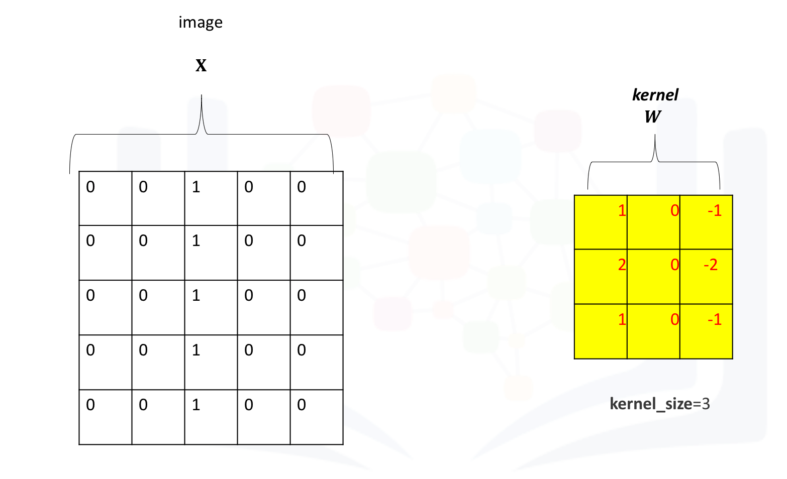
    Create a two-dimensional convolution object by using the constructor Conv2d, the parameter in_channels and out_channels will be used for this section, and the parameter kernel_size will be three.

    In [2]:
    Copied!
    conv = nn.Conv2d(in_channels=1, out_channels=1,kernel_size=3)
    conv
    
    conv = nn.Conv2d(in_channels=1, out_channels=1,kernel_size=3) conv
    Out[2]:
    Conv2d(1, 1, kernel_size=(3, 3), stride=(1, 1))

    Because the parameters in nn.Conv2d are randomly initialized and learned through training, give them some values.

    In [3]:
    Copied!
    conv.state_dict()['weight'][0][0]=torch.tensor([[1.0,0,-1.0],[2.0,0,-2.0],[1.0,0.0,-1.0]])
    conv.state_dict()['bias'][0]=0.0
    conv.state_dict()
    
    conv.state_dict()['weight'][0][0]=torch.tensor([[1.0,0,-1.0],[2.0,0,-2.0],[1.0,0.0,-1.0]]) conv.state_dict()['bias'][0]=0.0 conv.state_dict()
    Out[3]:
    OrderedDict([('weight',
                  tensor([[[[ 1.,  0., -1.],
                            [ 2.,  0., -2.],
                            [ 1.,  0., -1.]]]])),
                 ('bias', tensor([0.]))])

    Create a dummy tensor to represent an image. The shape of the image is (1,1,5,5) where:

    (number of inputs, number of channels, number of rows, number of columns )

    Set the third column to 1:

    In [4]:
    Copied!
    image=torch.zeros(1,1,5,5)
    image[0,0,:,2]=1
    image
    
    image=torch.zeros(1,1,5,5) image[0,0,:,2]=1 image
    Out[4]:
    tensor([[[[0., 0., 1., 0., 0.],
              [0., 0., 1., 0., 0.],
              [0., 0., 1., 0., 0.],
              [0., 0., 1., 0., 0.],
              [0., 0., 1., 0., 0.]]]])

    Call the object conv on the tensor image as an input to perform the convolution and assign the result to the tensor z.

    In [5]:
    Copied!
    z=conv(image)
    z
    
    z=conv(image) z
    Out[5]:
    tensor([[[[-4.,  0.,  4.],
              [-4.,  0.,  4.],
              [-4.,  0.,  4.]]]], grad_fn=<ConvolutionBackward0>)

    The following animation illustrates the process, the kernel performs at the element-level multiplication on every element in the image in the corresponding region. The values are then added together. The kernel is then shifted and the process is repeated.

    No description has been provided for this image

    Determining the Size of the Output

    The size of the output is an important parameter. In this lab, you will assume square images. For rectangular images, the same formula can be used in for each dimension independently.

    Let M be the size of the input and K be the size of the kernel. The size of the output is given by the following formula:

    $$M_{new}=M-K+1$$

    Create a kernel of size 2:

    In [6]:
    Copied!
    K=2
    conv1 = nn.Conv2d(in_channels=1, out_channels=1,kernel_size=K)
    conv1.state_dict()['weight'][0][0]=torch.tensor([[1.0,1.0],[1.0,1.0]])
    conv1.state_dict()['bias'][0]=0.0
    conv1.state_dict()
    conv1
    
    K=2 conv1 = nn.Conv2d(in_channels=1, out_channels=1,kernel_size=K) conv1.state_dict()['weight'][0][0]=torch.tensor([[1.0,1.0],[1.0,1.0]]) conv1.state_dict()['bias'][0]=0.0 conv1.state_dict() conv1
    Out[6]:
    Conv2d(1, 1, kernel_size=(2, 2), stride=(1, 1))

    Create an image of size 2:

    In [7]:
    Copied!
    M=4
    image1=torch.ones(1,1,M,M)
    
    M=4 image1=torch.ones(1,1,M,M)
    No description has been provided for this image

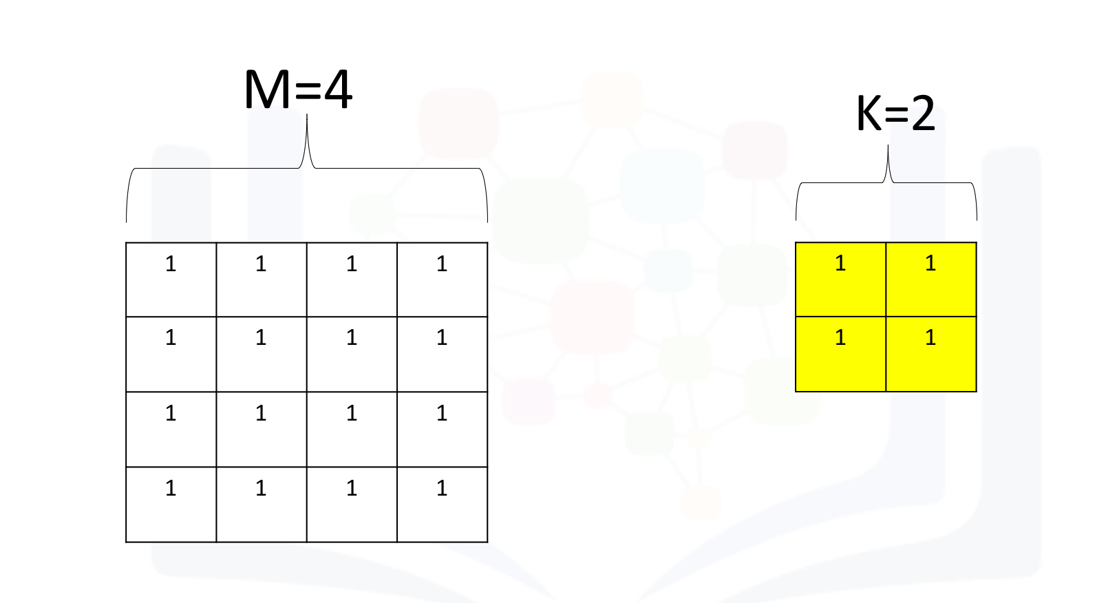
    The following equation provides the output:

    $$M_{new}=M-K+1$$ $$M_{new}=4-2+1$$ $$M_{new}=3$$

    The following animation illustrates the process: The first iteration of the kernel overlay of the images produces one output. As the kernel is of size K, there are M-K elements for the kernel to move in the horizontal direction. The same logic applies to the vertical direction.

    No description has been provided for this image

    Perform the convolution and verify the size is correct:

    In [8]:
    Copied!
    z1=conv1(image1)
    print("z1:",z1)
    print("shape:",z1.shape[2:4])
    
    z1=conv1(image1) print("z1:",z1) print("shape:",z1.shape[2:4])
    z1: tensor([[[[4., 4., 4.],
              [4., 4., 4.],
              [4., 4., 4.]]]], grad_fn=<ConvolutionBackward0>)
    shape: torch.Size([3, 3])
    

    Stride parameter

    The parameter stride changes the number of shifts the kernel moves per iteration. As a result, the output size also changes and is given by the following formula:

    $$M_{new}=\dfrac{M-K}{stride}+1$$

    Create a convolution object with a stride of 2:

    In [9]:
    Copied!
    conv3 = nn.Conv2d(in_channels=1, out_channels=1,kernel_size=2,stride=2)
    
    conv3.state_dict()['weight'][0][0]=torch.tensor([[1.0,1.0],[1.0,1.0]])
    conv3.state_dict()['bias'][0]=0.0
    conv3.state_dict()
    
    conv3 = nn.Conv2d(in_channels=1, out_channels=1,kernel_size=2,stride=2) conv3.state_dict()['weight'][0][0]=torch.tensor([[1.0,1.0],[1.0,1.0]]) conv3.state_dict()['bias'][0]=0.0 conv3.state_dict()
    Out[9]:
    OrderedDict([('weight',
                  tensor([[[[1., 1.],
                            [1., 1.]]]])),
                 ('bias', tensor([0.]))])

    For an image with a size of 4, calculate the output size:

    $$M_{new}=\dfrac{M-K}{stride}+1$$ $$M_{new}=\dfrac{4-2}{2}+1$$ $$M_{new}=2$$

    The following animation illustrates the process: The first iteration of the kernel overlay of the images produces one output. Because the kernel is of size K, there are M-K=2 elements. The stride is 2 because it will move 2 elements at a time. As a result, you divide M-K by the stride value 2:

    No description has been provided for this image

    Perform the convolution and verify the size is correct:

    In [10]:
    Copied!
    z3=conv3(image1)
    
    print("z3:",z3)
    print("shape:",z3.shape[2:4])
    
    z3=conv3(image1) print("z3:",z3) print("shape:",z3.shape[2:4])
    z3: tensor([[[[4., 4.],
              [4., 4.]]]], grad_fn=<ConvolutionBackward0>)
    shape: torch.Size([2, 2])
    

    Zero Padding

    As you apply successive convolutions, the image will shrink. You can apply zero padding to keep the image at a reasonable size, which also holds information at the borders.

    In addition, you might not get integer values for the size of the kernel. Consider the following image:

    In [11]:
    Copied!
    image1
    
    image1
    Out[11]:
    tensor([[[[1., 1., 1., 1.],
              [1., 1., 1., 1.],
              [1., 1., 1., 1.],
              [1., 1., 1., 1.]]]])

    Try performing convolutions with the kernel_size=2 and a stride=3. Use these values:

    $$M_{new}=\dfrac{M-K}{stride}+1$$ $$M_{new}=\dfrac{4-2}{3}+1$$ $$M_{new}=1.666$$

    In [12]:
    Copied!
    conv4 = nn.Conv2d(in_channels=1, out_channels=1,kernel_size=2,stride=3)
    conv4.state_dict()['weight'][0][0]=torch.tensor([[1.0,1.0],[1.0,1.0]])
    conv4.state_dict()['bias'][0]=0.0
    conv4.state_dict()
    z4=conv4(image1)
    print("z4:",z4)
    print("z4:",z4.shape[2:4])
    
    conv4 = nn.Conv2d(in_channels=1, out_channels=1,kernel_size=2,stride=3) conv4.state_dict()['weight'][0][0]=torch.tensor([[1.0,1.0],[1.0,1.0]]) conv4.state_dict()['bias'][0]=0.0 conv4.state_dict() z4=conv4(image1) print("z4:",z4) print("z4:",z4.shape[2:4])
    z4: tensor([[[[4.]]]], grad_fn=<ConvolutionBackward0>)
    z4: torch.Size([1, 1])
    

    You can add rows and columns of zeros around the image. This is called padding. In the constructor Conv2d, you specify the number of rows or columns of zeros that you want to add with the parameter padding.

    For a square image, you merely pad an extra column of zeros to the first column and the last column. Repeat the process for the rows. As a result, for a square image, the width and height is the original size plus 2 x the number of padding elements specified. You can then determine the size of the output after subsequent operations accordingly as shown in the following equation where you determine the size of an image after padding and then applying a convolutions kernel of size K.

    $$M'=M+2 \times padding$$ $$M_{new}=M'-K+1$$

    Consider the following example:

    In [13]:
    Copied!
    conv5 = nn.Conv2d(in_channels=1, out_channels=1,kernel_size=2,stride=3,padding=1)
    
    conv5.state_dict()['weight'][0][0]=torch.tensor([[1.0,1.0],[1.0,1.0]])
    conv5.state_dict()['bias'][0]=0.0
    conv5.state_dict()
    z5=conv5(image1)
    print("z5:",z5)
    print("z5:",z4.shape[2:4])
    
    conv5 = nn.Conv2d(in_channels=1, out_channels=1,kernel_size=2,stride=3,padding=1) conv5.state_dict()['weight'][0][0]=torch.tensor([[1.0,1.0],[1.0,1.0]]) conv5.state_dict()['bias'][0]=0.0 conv5.state_dict() z5=conv5(image1) print("z5:",z5) print("z5:",z4.shape[2:4])
    z5: tensor([[[[1., 2.],
              [2., 4.]]]], grad_fn=<ConvolutionBackward0>)
    z5: torch.Size([1, 1])
    
    In [ ]:
    Copied!


    The process is summarized in the following animation:

    No description has been provided for this image

    Practice Question

    A kernel of zeros with a kernel size=3 is applied to the following image:

    In [14]:
    Copied!
    Image=torch.randn((1,1,4,4))
    Image
    
    Image=torch.randn((1,1,4,4)) Image
    Out[14]:
    tensor([[[[-0.4460, -0.1425,  1.0888,  0.8292],
              [ 1.0301, -0.4119, -1.0132, -0.4925],
              [-1.1662, -0.5480,  1.7078,  0.0230],
              [-0.1644,  1.8086, -1.1509, -0.2585]]]])

    Question: Without using the function, determine what the outputs values are as each element:

    Double-click here for the solution.

    Question: Use the following convolution object to perform convolution on the tensor Image:

    In [15]:
    Copied!
    conv = nn.Conv2d(in_channels=1, out_channels=1,kernel_size=3)
    conv.state_dict()['weight'][0][0]=torch.tensor([[0,0,0],[0,0,0],[0,0.0,0]])
    conv.state_dict()['bias'][0]=0.0
    
    conv = nn.Conv2d(in_channels=1, out_channels=1,kernel_size=3) conv.state_dict()['weight'][0][0]=torch.tensor([[0,0,0],[0,0,0],[0,0.0,0]]) conv.state_dict()['bias'][0]=0.0

    Double-click here for the solution.

    Question: You have an image of size 4. The parameters are as follows kernel_size=2,stride=2. What is the size of the output?

    In [ ]:
    Copied!


    What's on your mind? Put it in the comments!

    June 3, 2025 June 3, 2025

    © 2025 DATAIDEA. All rights reserved. Built with ❤️ by Juma Shafara.