Welcome to our new Data Science resource site!

logo
Programming for Data Science
Activation & Pooling
Initializing search
    • Home
    • Python
    • Data Collection and Visualization
    • Machine Learning
    • Deep Learning
    • Time Series
    • Maths & Statistics
    • Extras
    • About
    • Home
      • Overview
      • End of Course Exercise
        • Outline
        • Introduction
        • Variables
        • Numbers
        • Strings
        • Operators
        • Containers
        • Flow Control
        • Advanced
        • Modules
        • File Handling
        • End of Course Exercise
        • Filter Function
        • Map Function
        • Reduce Function
        • NumPy Crash Course
        • Pandas Crash Course
        • Matplotlib Crash Course
      • NumPy Crash Course
      • Pandas Crash Course
      • Weather Data
      • Matplotlib Crash Course
      • Data Exploration Exercise
      • Handling Missing Data
      • Overview
      • Training Models
        • Introduction
        • Advanced
        • Feature Selection
        • Why Scaling
        • Feature Scaling (FPL)
        • Normalization and Standardization
      • Handling Missing Data
        • Classification Metrics
        • Regression Metrics
        • Pipelines
        • Hyperparameter Tuning
      • Introduction
        • 1D Tensors
        • 2D Tensors
        • Derivatives & Graphs
        • Simple Datasets
        • Pre-Built Datasets
        • Exercise
        • 1D Regression
        • One Parameter
        • Slope & Bias
        • Exercise
        • SGD
        • Mini-Batch GD
        • PyTorch Way
        • Training & Validation
        • Exercise
        • Multiple LR Prediction
        • Multiple LR Training
        • Multi-Target LR
        • Training Multiple Output
        • Exercise
        • Prediction
        • MSE Issues
        • Cross Entropy
        • Softmax
        • Exercise
        • Custom Datasets
        • DataLoaders
        • Transforms
        • Simple Hidden Layer
        • this is for exercises
        • XOR Problem
        • MNIST
        • Activation Functions
        • MNIST One Layer
        • MNIST Two Layer
        • Multiclass Spiral
        • Dropout Prediction
        • Dropout Regression
        • Initialization
        • Xavier Init
        • He Init
        • Momentum
        • NN with Momentum
        • Batch Normalization
        • Convolution Basics
        • Activation & Pooling
        • Multiple Channels
        • Simple CNN
        • CNN Small Image
        • CNN Batch Processing
      • Introduction
      • Analysis
      • Forecasting
      • Python Example
      • Overview
      • Eigen Values and Vectors
      • Descriptive Statistics
      • Inferential Statistics
      • Statistical Models
      • Hypothesis Testing
      • Customer Analysis
      • How KNN Works
      • Handling Imbalanced Data
      • Classification Metrics
      • License
      • ReadMe

    author: Juma Shafara date: "2024-08-12" title: Activation function and Maxpooling keywords: [Training Two Parameter, Mini-Batch Gradient Decent, Training Two Parameter Mini-Batch Gradient Decent] description: In this lab, you will learn two important components in building a convolutional neural network.

    Photo by DATAIDEA

    Objective for this Notebook

    1. Learn how to apply an activation function.
    2. Learn about max pooling

    Table of Contents

    In this lab, you will learn two important components in building a convolutional neural network. The first is applying an activation function, which is analogous to building a regular network. You will also learn about max pooling. Max pooling reduces the number of parameters and makes the network less susceptible to changes in the image.

  1. Activation Functions
  2. Max Pooling

  3. Estimated Time Needed: 25 min

    Don't Miss Any Updates!

    Before we continue, I have a humble request, to be among the first to hear about future updates of the course materials, simply enter your email below, follow us on (formally Twitter), or subscribe to our YouTube channel.

    Import the following libraries:

    In [1]:
    Copied!
    import torch 
    import torch.nn as nn
    import matplotlib.pyplot as plt
    import numpy as np
    from scipy import ndimage, misc
    
    import torch import torch.nn as nn import matplotlib.pyplot as plt import numpy as np from scipy import ndimage, misc

    Activation Functions

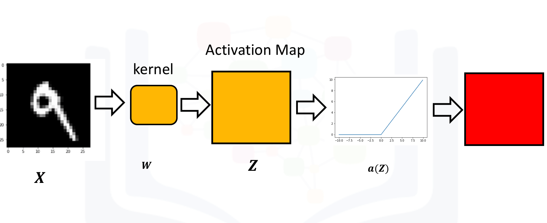
    Just like a neural network, you apply an activation function to the activation map as shown in the following image:

    No description has been provided for this image

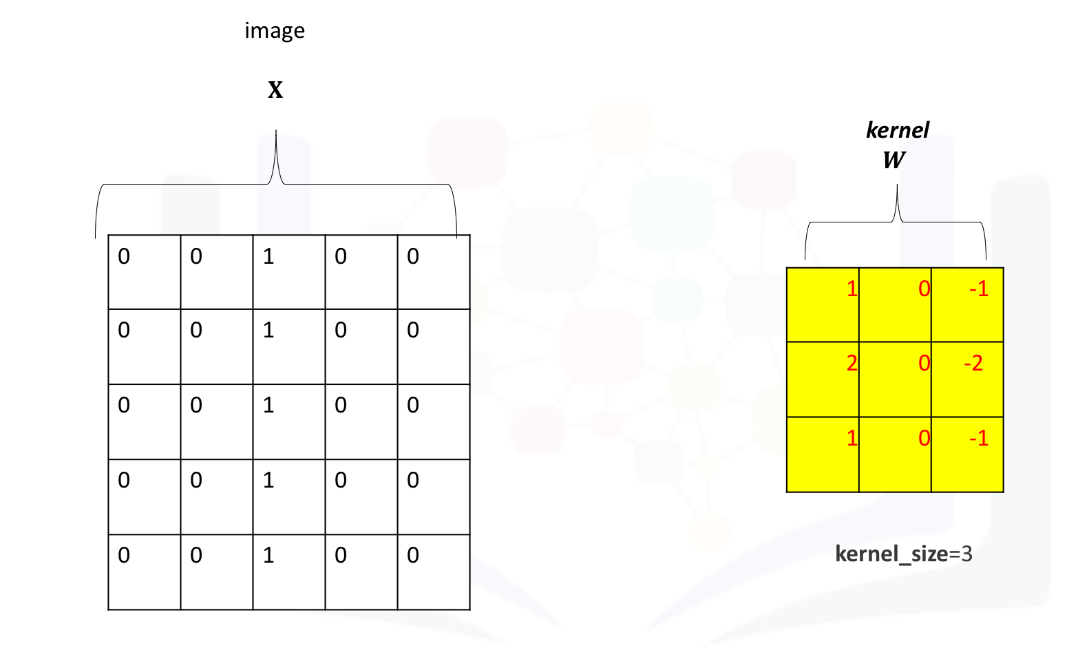
    Create a kernel and image as usual. Set the bias to zero:

    In [2]:
    Copied!
    conv = nn.Conv2d(in_channels=1, out_channels=1,kernel_size=3)
    Gx=torch.tensor([[1.0,0,-1.0],[2.0,0,-2.0],[1.0,0,-1.0]])
    conv.state_dict()['weight'][0][0]=Gx
    conv.state_dict()['bias'][0]=0.0
    conv.state_dict()
    
    conv = nn.Conv2d(in_channels=1, out_channels=1,kernel_size=3) Gx=torch.tensor([[1.0,0,-1.0],[2.0,0,-2.0],[1.0,0,-1.0]]) conv.state_dict()['weight'][0][0]=Gx conv.state_dict()['bias'][0]=0.0 conv.state_dict()
    Out[2]:
    OrderedDict([('weight',
                  tensor([[[[ 1.,  0., -1.],
                            [ 2.,  0., -2.],
                            [ 1.,  0., -1.]]]])),
                 ('bias', tensor([0.]))])
    In [3]:
    Copied!
    image=torch.zeros(1,1,5,5)
    image[0,0,:,2]=1
    image
    
    image=torch.zeros(1,1,5,5) image[0,0,:,2]=1 image
    Out[3]:
    tensor([[[[0., 0., 1., 0., 0.],
              [0., 0., 1., 0., 0.],
              [0., 0., 1., 0., 0.],
              [0., 0., 1., 0., 0.],
              [0., 0., 1., 0., 0.]]]])

    The following image shows the image and kernel:

    No description has been provided for this image

    Apply convolution to the image:

    In [4]:
    Copied!
    Z=conv(image)
    Z
    
    Z=conv(image) Z
    Out[4]:
    tensor([[[[-4.,  0.,  4.],
              [-4.,  0.,  4.],
              [-4.,  0.,  4.]]]], grad_fn=<ConvolutionBackward0>)

    Apply the activation function to the activation map. This will apply the activation function to each element in the activation map.

    In [5]:
    Copied!
    A=torch.relu(Z)
    A
    
    A=torch.relu(Z) A
    Out[5]:
    tensor([[[[0., 0., 4.],
              [0., 0., 4.],
              [0., 0., 4.]]]], grad_fn=<ReluBackward0>)
    In [6]:
    Copied!
    relu = nn.ReLU()
    relu(Z)
    
    relu = nn.ReLU() relu(Z)
    Out[6]:
    tensor([[[[0., 0., 4.],
              [0., 0., 4.],
              [0., 0., 4.]]]], grad_fn=<ReluBackward0>)

    The process is summarized in the the following figure. The Relu function is applied to each element. All the elements less than zero are mapped to zero. The remaining components do not change.

    No description has been provided for this image

    Max Pooling

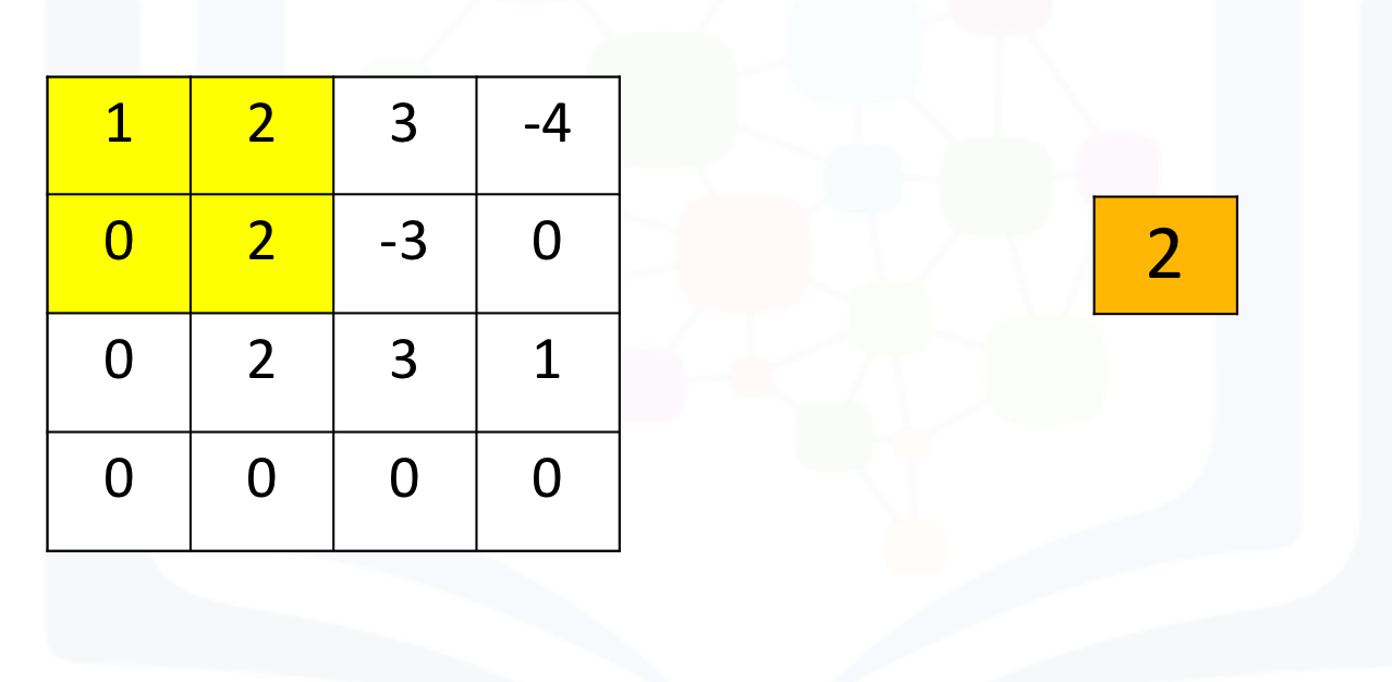
    Consider the following image:

    In [7]:
    Copied!
    image1=torch.zeros(1,1,4,4)
    image1[0,0,0,:]=torch.tensor([1.0,2.0,3.0,-4.0])
    image1[0,0,1,:]=torch.tensor([0.0,2.0,-3.0,0.0])
    image1[0,0,2,:]=torch.tensor([0.0,2.0,3.0,1.0])
    
    image1
    
    image1=torch.zeros(1,1,4,4) image1[0,0,0,:]=torch.tensor([1.0,2.0,3.0,-4.0]) image1[0,0,1,:]=torch.tensor([0.0,2.0,-3.0,0.0]) image1[0,0,2,:]=torch.tensor([0.0,2.0,3.0,1.0]) image1
    Out[7]:
    tensor([[[[ 1.,  2.,  3., -4.],
              [ 0.,  2., -3.,  0.],
              [ 0.,  2.,  3.,  1.],
              [ 0.,  0.,  0.,  0.]]]])

    Max pooling simply takes the maximum value in each region. Consider the following image. For the first region, max pooling simply takes the largest element in a yellow region.

    No description has been provided for this image

    The region shifts, and the process is repeated. The process is similar to convolution and is demonstrated in the following figure:

    No description has been provided for this image

    Create a maxpooling object in 2d as follows and perform max pooling as follows:

    In [8]:
    Copied!
    max1=torch.nn.MaxPool2d(2,stride=1)
    max1(image1)
    
    max1=torch.nn.MaxPool2d(2,stride=1) max1(image1)
    Out[8]:
    tensor([[[[2., 3., 3.],
              [2., 3., 3.],
              [2., 3., 3.]]]])

    If the stride is set to None (its defaults setting), the process will simply take the maximum in a prescribed area and shift over accordingly as shown in the following figure:

    No description has been provided for this image

    Here's the code in Pytorch:

    What's on your mind? Put it in the comments!

    June 3, 2025 June 3, 2025

    © 2025 DATAIDEA. All rights reserved. Built with ❤️ by Juma Shafara.