Overview of Machine Learning

Machine learning (ML) is a branch of artificial intelligence (AI) and computer science that focuses on using data and algorithms to enable AI to imitate the way that humans learn, and gradually improve.

Keywords

What is Machine Learning

Photo by DATAIDEA

1. Introduction to Machine Learning

Machine learning (ML) is a branch of artificial intelligence that involves training algorithms to make predictions or decisions based on data. It’s widely used in many fields, such as healthcare, finance, and marketing.

2. Types of Machine Learning

• Supervised Learning: Learn from labeled data.
• Unsupervised Learning: Discover patterns in unlabeled data.
• Reinforcement Learning: Agents learn to make decisions by interacting with the environment.

3. Key Concepts in Machine Learning

• Feature: A measurable property of the data.
• Label: The target variable (what you’re predicting).
• Training Set: The data used to train the model.
• Test Set: The data used to evaluate the model’s performance.

4. Steps in a Machine Learning Workflow

1. Data Collection
2. Data Preprocessing
3. Feature Engineering
4. Model Selection
5. Model Training
6. Model Evaluation
7. Hyperparameter Tuning

---

5. Real-world Application with Iris Dataset

(a) Data Loading

We will load the Iris dataset using sklearn.datasets.

import pandas as pd
from sklearn.datasets import load_iris

# Load Iris dataset
iris = load_iris()
X = pd.DataFrame(iris.data, columns=iris.feature_names)
y = pd.Series(iris.target, name='species')

# Display the first 5 rows of the dataset
X.head()

	sepal length (cm)	sepal width (cm)	petal length (cm)	petal width (cm)
0	5.1	3.5	1.4	0.2
1	4.9	3.0	1.4	0.2
2	4.7	3.2	1.3	0.2
3	4.6	3.1	1.5	0.2
4	5.0	3.6	1.4	0.2

(b) Data Preprocessing

We check for missing values, and split the data into training and testing sets.

from sklearn.model_selection import train_test_split

# Split data into train and test sets (80% train, 20% test)
X_train, X_test, y_train, y_test = train_test_split(X, y, test_size=0.25, random_state=42)

# Check for missing values
print(X.isnull().sum())

sepal length (cm)    0
sepal width (cm)     0
petal length (cm)    0
petal width (cm)     0
dtype: int64

(c) Exploratory Data Analysis (EDA)

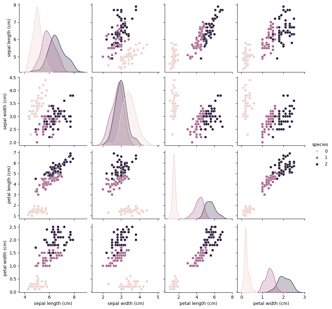
We’ll visualize the relationship between features and the target label.

import seaborn as sns
import matplotlib.pyplot as plt

# Pairplot to visualize relationships between features
sns.pairplot(pd.concat([X, y], axis=1), hue="species")
plt.show()

(d) Model Training

We will train a Logistic Regression model, which is a simple yet effective supervised learning algorithm.

from sklearn.linear_model import LogisticRegression

# Initialize and train the model
model = LogisticRegression()
model.fit(X_train, y_train)

LogisticRegression()

In a Jupyter environment, please rerun this cell to show the HTML representation or trust the notebook.
On GitHub, the HTML representation is unable to render, please try loading this page with nbviewer.org.

(e) Model Evaluation

We evaluate the model’s performance using accuracy and confusion matrix.

from sklearn.metrics import accuracy_score, confusion_matrix

# Predict on the test set
y_pred = model.predict(X_test)

# Evaluate the model
accuracy = accuracy_score(y_test, y_pred)
conf_matrix = confusion_matrix(y_test, y_pred)

print(f"Accuracy: {accuracy}")
print("Confusion Matrix:")
print(conf_matrix)

Accuracy: 1.0
Confusion Matrix:
[[15  0  0]
 [ 0 11  0]
 [ 0  0 12]]

(f) Hyperparameter Tuning

We use GridSearchCV to find the best hyperparameters for our model.

from sklearn.model_selection import GridSearchCV

# Define parameter grid
param_grid = {'C': [0.1, 1, 10], 'solver': ['lbfgs', 'liblinear']}

# Grid search
grid_search = GridSearchCV(LogisticRegression(max_iter=200), param_grid, cv=5)
grid_search.fit(X_train, y_train)

# Best parameters
print("Best Parameters: ", grid_search.best_params_)

Best Parameters:  {'C': 1, 'solver': 'lbfgs'}

(g) Conclusion

Congratulations on reaching the end of the tutorial, with the simple Logistic Regression model, we achieved a good accuracy on the Iris dataset. This example shows how to:

• Load and preprocess data
• Perform EDA
• Train and evaluate a model
• Tune hyperparameters for better performance

What’s on your mind? Put it in the comments!