# Import the libraries we need for this lab

import numpy as np
import matplotlib.pyplot as plt
from mpl_toolkits import mplot3d
import torch
from torch.utils.data import Dataset, DataLoader
import torch.nn as nnLogistic Regression and Bad Initialization Value
In this lab, you will see what happens when you use the root mean square error cost or total loss function and select a bad initialization value for the parameter values.
Keywords
Training Two Parameter, Mini-Batch Gradient Decent, Training Two Parameter Mini-Batch Gradient Decent

Objective
- How bad initialization value can affects the accuracy of model. .
Table of Contents
In this lab, you will see what happens when you use the root mean square error cost or total loss function and select a bad initialization value for the parameter values.
- Make Some Data
- Create the Model and Cost Function the PyTorch way
- Train the Model:Batch Gradient Descent
Estimated Time Needed: 30 min
Preparation
We’ll need the following libraries:
Helper functions
The class plot_error_surfaces is just to help you visualize the data space and the Parameter space during training and has nothing to do with Pytorch.
# Create class for plotting and the function for plotting
class plot_error_surfaces(object):
# Construstor
def __init__(self, w_range, b_range, X, Y, n_samples = 30, go = True):
W = np.linspace(-w_range, w_range, n_samples)
B = np.linspace(-b_range, b_range, n_samples)
w, b = np.meshgrid(W, B)
Z = np.zeros((30, 30))
count1 = 0
self.y = Y.numpy()
self.x = X.numpy()
for w1, b1 in zip(w, b):
count2 = 0
for w2, b2 in zip(w1, b1):
Z[count1, count2] = np.mean((self.y - (1 / (1 + np.exp(-1*w2 * self.x - b2)))) ** 2)
count2 += 1
count1 += 1
self.Z = Z
self.w = w
self.b = b
self.W = []
self.B = []
self.LOSS = []
self.n = 0
if go == True:
plt.figure()
plt.figure(figsize=(7.5, 5))
plt.axes(projection='3d').plot_surface(self.w, self.b, self.Z, rstride=1, cstride=1, cmap='viridis', edgecolor='none')
plt.title('Loss Surface')
plt.xlabel('w')
plt.ylabel('b')
plt.show()
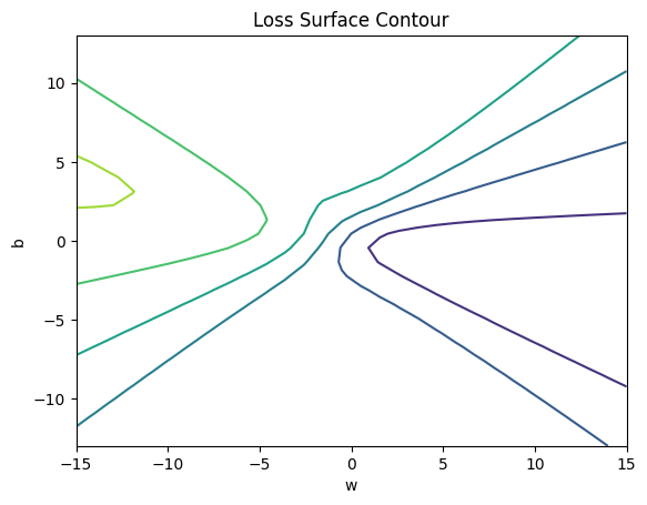
plt.figure()
plt.title('Loss Surface Contour')
plt.xlabel('w')
plt.ylabel('b')
plt.contour(self.w, self.b, self.Z)
plt.show()
# Setter
def set_para_loss(self, model, loss):
self.n = self.n + 1
self.W.append(list(model.parameters())[0].item())
self.B.append(list(model.parameters())[1].item())
self.LOSS.append(loss)
# Plot diagram
def final_plot(self):
ax = plt.axes(projection='3d')
ax.plot_wireframe(self.w, self.b, self.Z)
ax.scatter(self.W, self.B, self.LOSS, c='r', marker='x', s=200, alpha=1)
plt.figure()
plt.contour(self.w, self.b, self.Z)
plt.scatter(self.W, self.B, c='r', marker='x')
plt.xlabel('w')
plt.ylabel('b')
plt.show()
# Plot diagram
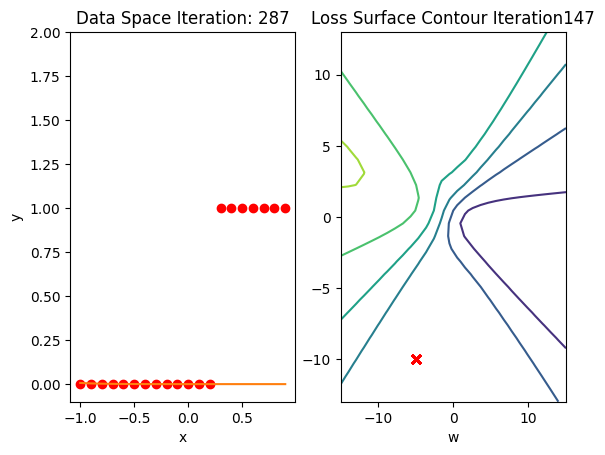
def plot_ps(self):
plt.subplot(121)
plt.ylim
plt.plot(self.x, self.y, 'ro', label="training points")
plt.plot(self.x, self.W[-1] * self.x + self.B[-1], label="estimated line")
plt.plot(self.x, 1 / (1 + np.exp(-1 * (self.W[-1] * self.x + self.B[-1]))), label='sigmoid')
plt.xlabel('x')
plt.ylabel('y')
plt.ylim((-0.1, 2))
plt.title('Data Space Iteration: ' + str(self.n))
plt.show()
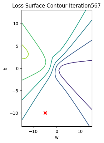
plt.subplot(122)
plt.contour(self.w, self.b, self.Z)
plt.scatter(self.W, self.B, c='r', marker='x')
plt.title('Loss Surface Contour Iteration' + str(self.n))
plt.xlabel('w')
plt.ylabel('b')
# Plot the diagram
def PlotStuff(X, Y, model, epoch, leg=True):
plt.plot(X.numpy(), model(X).detach().numpy(), label=('epoch ' + str(epoch)))
plt.plot(X.numpy(), Y.numpy(), 'r')
if leg == True:
plt.legend()
else:
passSet the random seed:
# Set random seed

torch.manual_seed(0)
<torch._C.Generator at 0x7c89b4a521f0>Get Some Data
Create the Data class
# Create the data class

class Data(Dataset):

    # Constructor
    def __init__(self):
        self.x = torch.arange(-1, 1, 0.1).view(-1, 1)
        self.y = torch.zeros(self.x.shape[0], 1)
        self.y[self.x[:, 0] > 0.2] = 1
        self.len = self.x.shape[0]

    # Getter
    def __getitem__(self, index):
        return self.x[index], self.y[index]

    # Get Length
    def __len__(self):
        return self.len
Make Data object
# Create Data object

data_set = Data()
Create the Model and Total Loss Function (Cost)
Create a custom module for logistic regression:
# Create logistic_regression class

class logistic_regression(nn.Module):

    # Constructor
    def __init__(self, n_inputs):
        super(logistic_regression, self).__init__()
        self.linear = nn.Linear(n_inputs, 1)

    # Prediction
    def forward(self, x):
        yhat = torch.sigmoid(self.linear(x))
        return yhat
Create a logistic regression object or model:
# Create the logistic_regression result

model = logistic_regression(1)
Replace the random initialized variable values with some predetermined values that will not converge:
# Set the weight and bias

model.state_dict() ['linear.weight'].data[0] = torch.tensor([[-5]])
model.state_dict() ['linear.bias'].data[0] = torch.tensor([[-10]])
print("The parameters: ", model.state_dict())
The parameters: OrderedDict({'linear.weight': tensor([[-5.]]), 'linear.bias': tensor([-10.])})Create a plot_error_surfaces object to visualize the data space and the parameter space during training:
# Create the plot_error_surfaces object

get_surface = plot_error_surfaces(15, 13, data_set[:][0], data_set[:][1], 30)
<Figure size 640x480 with 0 Axes>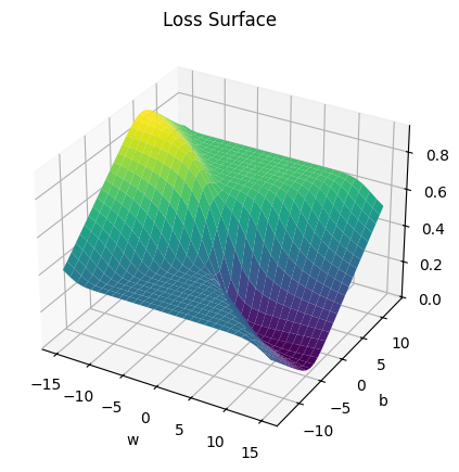
Define the dataloader, the cost or criterion function, the optimizer:
# Create dataloader object, crierion function and optimizer.

trainloader = DataLoader(dataset=data_set, batch_size=3)
criterion_rms = nn.MSELoss()
learning_rate = 2
optimizer = torch.optim.SGD(model.parameters(), lr=learning_rate)
Train the Model via Batch Gradient Descent
Train the model
# Train the model

def train_model(epochs):
    for epoch in range(epochs):
        for x, y in trainloader:
            yhat = model(x)
            loss = criterion_rms(yhat, y)
            optimizer.zero_grad()
            loss.backward()
            optimizer.step()
            get_surface.set_para_loss(model, loss.tolist())
        if epoch % 20 == 0:
            get_surface.plot_ps()

train_model(100)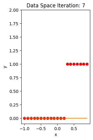
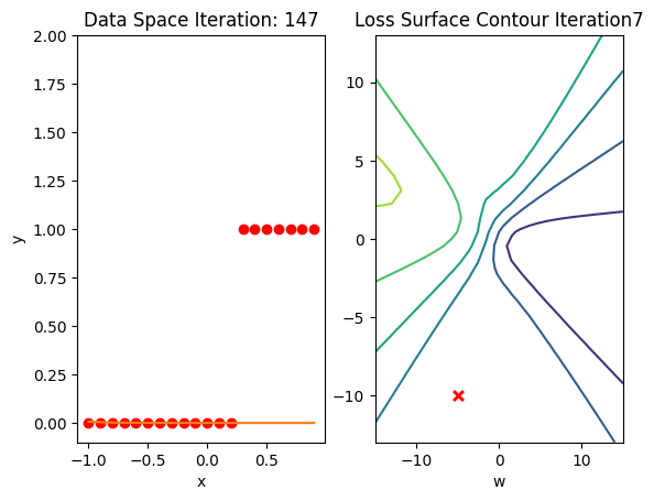


Get the actual class of each sample and calculate the accuracy on the test data:
# Make the Prediction

yhat = model(data_set.x)
label = yhat > 0.5
print("The accuracy: ", torch.mean((label == data_set.y.type(torch.ByteTensor)).type(torch.float)))
The accuracy: tensor(0.6500)Accuracy is 60% compared to 100% in the last lab using a good Initialization value.