# Import libraries we need for this lab, and set the random seed

from torch import nn
import torch
import numpy as np
import matplotlib.pyplot as plt
from torch import nn,optimTraining and Validation Data
How to use learning rate hyperparameter to improve your model result
Keywords
T Training and Validation Data, Create a Linear Regression Object, Data Loader, Criterion Function, Different learning rates, Data Structures, different Hyperparameters, Train different models for different Hyperparameters

Linear regression: Training and Validation Data
Objective
- How to use learning rate hyperparameter to improve your model result.
Table of Contents
In this lab, you will learn to select the best learning rate by using validation data.
- Make Some Data
- Create a Linear Regression Object, Data Loader and Criterion Function
- Different learning rates and Data Structures to Store results for Different Hyperparameters
- Train different modules for different Hyperparameters
- View Results
Estimated Time Needed: 30 min
Preparation
We’ll need the following libraries and set the random seed.
Make Some Data
First, we’ll create some artificial data in a dataset class. The class will include the option to produce training data or validation data. The training data will include outliers.
# Create Data class

from torch.utils.data import Dataset, DataLoader

class Data(Dataset):

    # Constructor
    def __init__(self, train = True):
            self.x = torch.arange(-3, 3, 0.1).view(-1, 1)
            self.f = -3 * self.x + 1
            self.y = self.f + 0.1 * torch.randn(self.x.size())
            self.len = self.x.shape[0]

            #outliers
            if train == True:
                self.y[0] = 0
                self.y[50:55] = 20
            else:
                pass

    # Getter
    def __getitem__(self, index):
        return self.x[index], self.y[index]

    # Get Length
    def __len__(self):
        return self.len
Create two objects: one that contains training data and a second that contains validation data. Assume that the training data has the outliers.
# Create training dataset and validation dataset

train_data = Data()
val_data = Data(train = False)
Overlay the training points in red over the function that generated the data. Notice the outliers at x=-3 and around x=2:
# Plot out training points

plt.plot(train_data.x.numpy(), train_data.y.numpy(), 'xr',label="training data ")
plt.plot(train_data.x.numpy(), train_data.f.numpy(),label="true function  ")
plt.xlabel('x')
plt.ylabel('y')
plt.legend()
plt.show()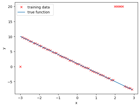
Create a Linear Regression Object, Data Loader, and Criterion Function
# Create Linear Regression Class

from torch import nn

class linear_regression(nn.Module):

    # Constructor
    def __init__(self, input_size, output_size):
        super(linear_regression, self).__init__()
        self.linear = nn.Linear(input_size, output_size)

    # Prediction function
    def forward(self, x):
        yhat = self.linear(x)
        return yhat
Create the criterion function and a DataLoader object:
# Create MSELoss function and DataLoader

criterion = nn.MSELoss()
trainloader = DataLoader(dataset = train_data, batch_size = 1)
Different learning rates and Data Structures to Store results for different Hyperparameters
Create a list with different learning rates and a tensor (can be a list) for the training and validating cost/total loss. Include the list MODELS, which stores the training model for every value of the learning rate.
# Create Learning Rate list, the error lists and the MODELS list

learning_rates=[0.0001, 0.001, 0.01, 0.1]

train_error=torch.zeros(len(learning_rates))
validation_error=torch.zeros(len(learning_rates))

MODELS=[]
Train different models for different Hyperparameters
Try different values of learning rates, perform stochastic gradient descent, and save the results on the training data and validation data. Finally, save each model in a list.
# Define the train model function and train the model

def train_model_with_lr (iter, lr_list):

    # iterate through different learning rates
    for i, lr in enumerate(lr_list):
        model = linear_regression(1, 1)
        optimizer = optim.SGD(model.parameters(), lr = lr)
        for epoch in range(iter):
            for x, y in trainloader:
                yhat = model(x)
                loss = criterion(yhat, y)
                optimizer.zero_grad()
                loss.backward()
                optimizer.step()

        # train data
        Yhat = model(train_data.x)
        train_loss = criterion(Yhat, train_data.y)
        train_error[i] = train_loss.item()

        # validation data
        Yhat = model(val_data.x)
        val_loss = criterion(Yhat, val_data.y)
        validation_error[i] = val_loss.item()
        MODELS.append(model)

train_model_with_lr(10, learning_rates)
View the Results
Plot the training loss and validation loss for each learning rate:
# Plot the training loss and validation loss

plt.semilogx(np.array(learning_rates), train_error.numpy(), label = 'training loss/total Loss')
plt.semilogx(np.array(learning_rates), validation_error.numpy(), label = 'validation cost/total Loss')
plt.ylabel('Cost\ Total Loss')
plt.xlabel('learning rate')
plt.legend()
plt.show()
<>:5: SyntaxWarning: invalid escape sequence '\ '
<>:5: SyntaxWarning: invalid escape sequence '\ '
/tmp/ipykernel_80257/980418342.py:5: SyntaxWarning: invalid escape sequence '\ '
plt.ylabel('Cost\ Total Loss')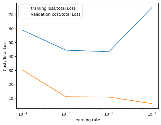
Produce a prediction by using the validation data for each model:
# Plot the predictions

i = 0
for model, learning_rate in zip(MODELS, learning_rates):
    yhat = model(val_data.x)
    plt.plot(val_data.x.numpy(), yhat.detach().numpy(), label = 'lr:' + str(learning_rate))
    print('i', yhat.detach().numpy()[0:3])
plt.plot(val_data.x.numpy(), val_data.f.numpy(), 'or', label = 'validation data')
plt.xlabel('x')
plt.ylabel('y')
plt.legend()
plt.show()
i [[0.05840436]
[0.06799743]
[0.0775905 ]]
i [[5.4587383]
[5.343816 ]
[5.2288933]]
i [[6.5484743]
[6.4158573]
[6.28324 ]]
i [[14.55032 ]
[14.1119585]
[13.673596 ]]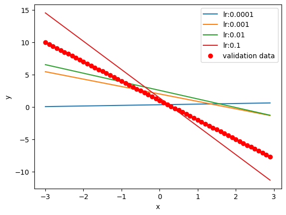
Practice
The object good_model is the best performing model. Use the train loader to get the data samples x and y. Produce an estimate for yhat and print it out for every sample in a for a loop. Compare it to the actual prediction y.
Double-click here for the solution.
Back to top