# These are the libraries we are going to use in the lab.

import numpy as np
import matplotlib.pyplot as plt
from mpl_toolkits import mplot3dLinear regression 1D, Training Two Parameters
In this lab, you will train a model with PyTorch by using the data that we created. The model will have the slope and bias.

Objective
- How to train the model and visualize the loss results.
Table of Contents
In this lab, you will train a model with PyTorch by using the data that we created. The model will have the slope and bias. And we will review how to make a prediction in several different ways by using PyTorch.
Estimated Time Needed: 20 min
Preparation
We’ll need the following libraries:
The class plot_error_surfaces is just to help you visualize the data space and the parameter space during training and has nothing to do with PyTorch.
Make Some Data
Import PyTorch:
# Import PyTorch library

import torch
Start with generating values from -3 to 3 that create a line with a slope of 1 and a bias of -1. This is the line that you need to estimate.
# Create f(X) with a slope of 1 and a bias of -1

X = torch.arange(-3, 3, 0.1).view(-1, 1)
f = 1 * X - 1
Now, add some noise to the data:
# Add noise

Y = f + 0.1 * torch.randn(X.size())
Plot the line and Y with noise:
# Plot out the line and the points with noise

plt.plot(X.numpy(), Y.numpy(), 'rx', label = 'y')
plt.plot(X.numpy(), f.numpy(), label = 'f')
plt.xlabel('x')
plt.ylabel('y')
plt.legend()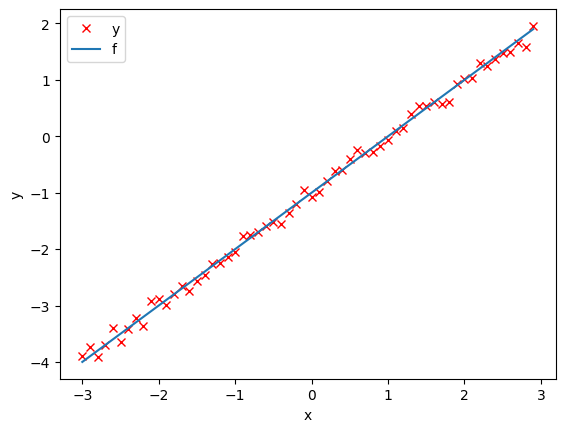
Create the Model and Cost Function (Total Loss)
Define the forward function:
# Define the forward function

def forward(x):
    return w * x + b
Define the cost or criterion function (MSE):
# Define the MSE Loss function
def criterion(yhat,y):
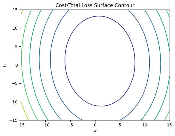
return torch.mean((yhat-y)**2)Create a plot_error_surfaces object to visualize the data space and the parameter space during training:
# Create plot_error_surfaces for viewing the data

get_surface = plot_error_surfaces(15, 15, X, Y, 30)
<Figure size 640x480 with 0 Axes>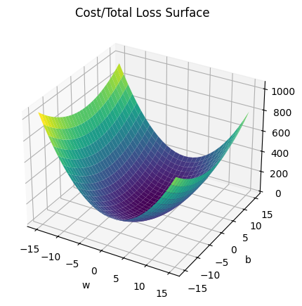
Train the Model
Create model parameters w, b by setting the argument requires_grad to True because we must learn it using the data.
# Define the parameters w, b for y = wx + b

w = torch.tensor(-15.0, requires_grad = True)
b = torch.tensor(-10.0, requires_grad = True)
Set the learning rate to 0.1 and create an empty list LOSS for storing the loss for each iteration.
# Define learning rate and create an empty list for containing the loss for each iteration.

lr = 0.1
LOSS = []
Define train_model function for train the model.
# The function for training the model
def train_model(iter):
# Loop
for epoch in range(iter):
# make a prediction
Yhat = forward(X)
# calculate the loss
loss = criterion(Yhat, Y)
# Section for plotting
get_surface.set_para_loss(w.data.tolist(), b.data.tolist(), loss.tolist())
if epoch % 3 == 0:
get_surface.plot_ps()
# store the loss in the list LOSS
LOSS.append(loss.item())
# backward pass: compute gradient of the loss with respect to all the learnable parameters
loss.backward()
# update parameters slope and bias
w.data = w.data - lr * w.grad.data
b.data = b.data - lr * b.grad.data
# zero the gradients before running the backward pass
w.grad.data.zero_()
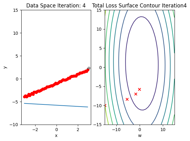
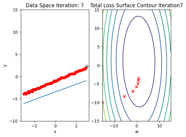
b.grad.data.zero_()Run 15 iterations of gradient descent: bug data space is 1 iteration ahead of parameter space
# Train the model with 15 iterations

train_model(15)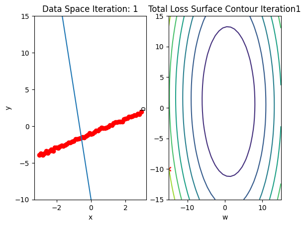

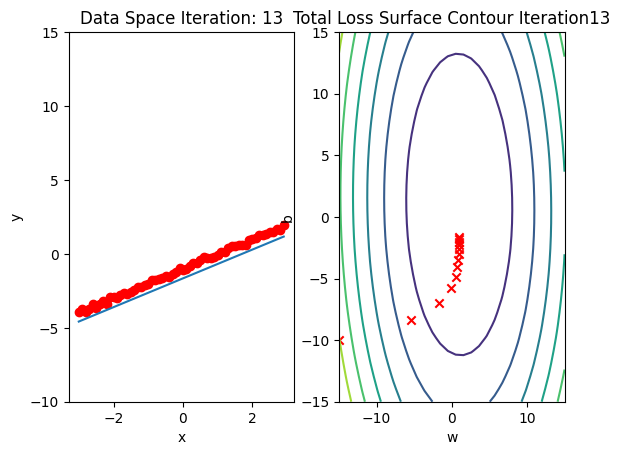
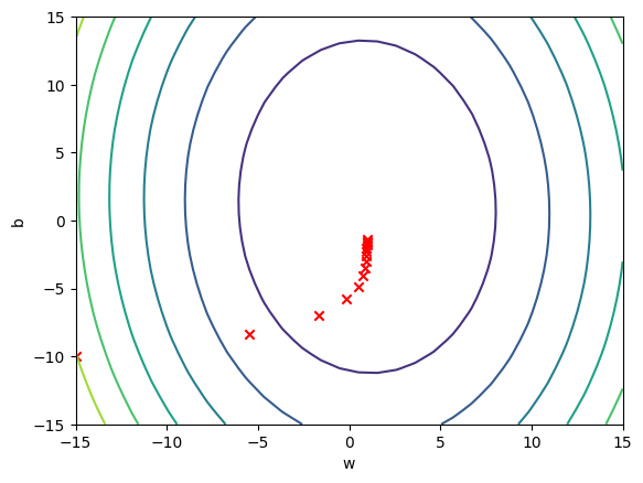
Plot total loss/cost surface with loss values for different parameters in red:
# Plot out the Loss Result


get_surface.final_plot()
plt.plot(LOSS)
plt.tight_layout()
plt.xlabel("Epoch/Iterations")
plt.ylabel("Cost")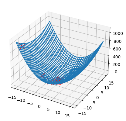
Text(38.347222222222214, 0.5, 'Cost')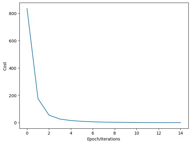
Practice
Experiment using s learning rates 0.2 and width the following parameters. Run 15 iterations.
# Practice: train and plot the result with lr = 0.2 and the following parameters

w = torch.tensor(-15.0, requires_grad = True)
b = torch.tensor(-10.0, requires_grad = True)
lr = 0.2
LOSS2 = []
Double-click here for the solution.
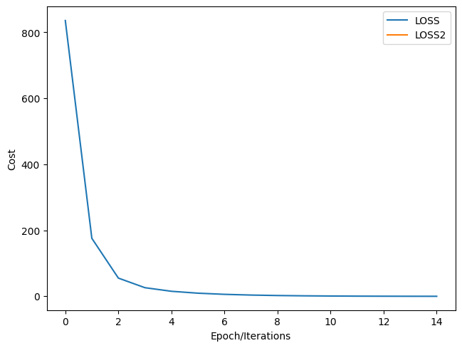
Plot the LOSS and LOSS2
# Practice: Plot the LOSS and LOSS2 in order to compare the Total Loss

# Type your code here
plt.plot(LOSS, label = "LOSS")
plt.plot(LOSS2, label = "LOSS2")
plt.tight_layout()
plt.xlabel("Epoch/Iterations")
plt.ylabel("Cost")
plt.legend()