# Import the libraries we need for this lab

import torch
import torch.nn as nn
from torch import sigmoid
import matplotlib.pylab as plt
import numpy as np
torch.manual_seed(0)
<torch._C.Generator at 0x7c4f98773170>Training Two Parameter, Mini-Batch Gradient Decent, Training Two Parameter Mini-Batch Gradient Decent

In this lab, you will use a single-layer neural network to classify non linearly seprable data in 1-Ddatabase.
Estimated Time Needed: 25 min
We’ll need the following libraries
# Import the libraries we need for this lab
import torch
import torch.nn as nn
from torch import sigmoid
import matplotlib.pylab as plt
import numpy as np
torch.manual_seed(0)<torch._C.Generator at 0x7c4f98773170>Used for plotting the model
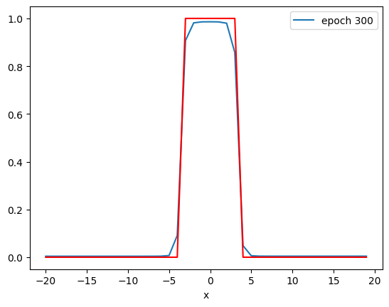
# The function for plotting the model
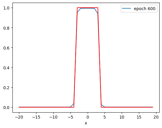
def PlotStuff(X, Y, model, epoch, leg=True):
plt.plot(X.numpy(), model(X).detach().numpy(), label=('epoch ' + str(epoch)))
plt.plot(X.numpy(), Y.numpy(), 'r')
plt.xlabel('x')
if leg == True:
plt.legend()
else:
passDefine the activations and the output of the first linear layer as an attribute. Note that this is not good practice.
# Define the class Net

class Net(nn.Module):

    # Constructor
    def __init__(self, D_in, H, D_out):
        super(Net, self).__init__()
        # hidden layer
        self.linear1 = nn.Linear(D_in, H)
        self.linear2 = nn.Linear(H, D_out)
        # Define the first linear layer as an attribute, this is not good practice
        self.a1 = None
        self.l1 = None
        self.l2=None

    # Prediction
    def forward(self, x):
        self.l1 = self.linear1(x)
        self.a1 = sigmoid(self.l1)
        self.l2=self.linear2(self.a1)
        yhat = sigmoid(self.linear2(self.a1))
        return yhat
Define the training function:
# Define the training function
def train(Y, X, model, optimizer, criterion, epochs=1000):
cost = []
total=0
for epoch in range(epochs):
total=0
for y, x in zip(Y, X):
yhat = model(x)
loss = criterion(yhat, y)
loss.backward()
optimizer.step()
optimizer.zero_grad()
#cumulative loss
total+=loss.item()
cost.append(total)
if epoch % 300 == 0:
PlotStuff(X, Y, model, epoch, leg=True)
plt.show()
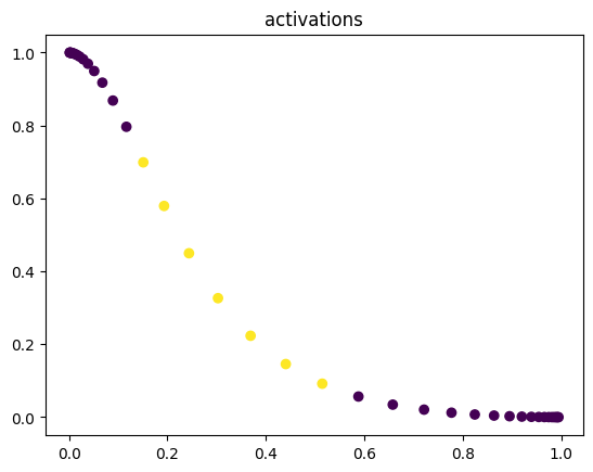
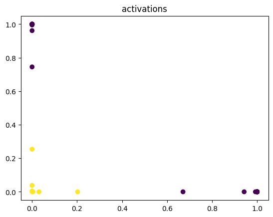
model(X)
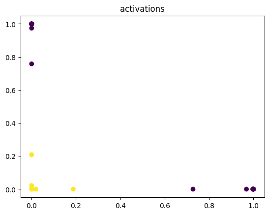
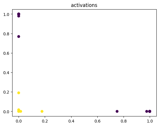
plt.scatter(model.a1.detach().numpy()[:, 0], model.a1.detach().numpy()[:, 1], c=Y.numpy().reshape(-1))
plt.title('activations')
plt.show()
return cost# Make some data
X = torch.arange(-20, 20, 1).view(-1, 1).type(torch.FloatTensor)
Y = torch.zeros(X.shape[0])
Y[(X[:, 0] > -4) & (X[:, 0] < 4)] = 1.0Create the Cross-Entropy loss function:
# The loss function

def criterion_cross(outputs, labels):
    out = -1 * torch.mean(labels * torch.log(outputs) + (1 - labels) * torch.log(1 - outputs))
    return out
Define the Neural Network, Optimizer, and Train the Model:
# Train the model
# size of input
D_in = 1
# size of hidden layer
H = 2
# number of outputs
D_out = 1
# learning rate
learning_rate = 0.1
# create the model
model = Net(D_in, H, D_out)
#optimizer
optimizer = torch.optim.SGD(model.parameters(), lr=learning_rate)
#train the model usein
cost_cross = train(Y, X, model, optimizer, criterion_cross, epochs=1000)
#plot the loss
plt.plot(cost_cross)
plt.xlabel('epoch')
plt.title('cross entropy loss')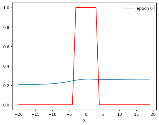

Text(0.5, 1.0, 'cross entropy loss')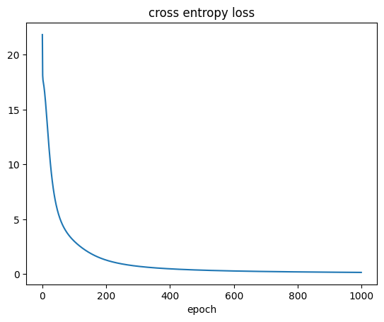
By examining the output of the activation, you see by the 600th epoch that the data has been mapped to a linearly separable space.
we can make a prediction for a arbitrary one tensors
x=torch.tensor([0.0])
yhat=model(x)
yhat
we can make a prediction for some arbitrary one tensors
X_=torch.tensor([[0.0],[2.0],[3.0]])
Yhat=model(X_)
Yhat
we can threshold the predication
Yhat=Yhat>0.5
YhatRepeat the previous steps above by using the MSE cost or total loss:
# Practice: Train the model with MSE Loss Function

# Type your code here
Double-click here for the solution.