# These are the libraries will be used for this lab.

import numpy as np
import matplotlib.pyplot as pltLinear Regression 1D, Training One Parameter
In this lab, you will train a model with PyTorch by using data that you created

Linear Regression 1D: Training One Parameter
Objective
- How to create cost or criterion function using MSE (Mean Square Error).
Table of Contents
In this lab, you will train a model with PyTorch by using data that you created. The model only has one parameter: the slope.
Estimated Time Needed: 20 min
Preparation
The following are the libraries we are going to use for this lab.
The class plot_diagram helps us to visualize the data space and the parameter space during training and has nothing to do with PyTorch.
# The class for plotting

class plot_diagram():

    # Constructor
    def __init__(self, X, Y, w, stop, go = False):
        start = w.data
        self.error = []
        self.parameter = []
        self.X = X.numpy()
        self.Y = Y.numpy()
        self.parameter_values = torch.arange(start, stop)
        self.Loss_function = [criterion(forward(X), Y) for w.data in self.parameter_values]
        w.data = start

    # Executor
    def __call__(self, Yhat, w, error, n):
        self.error.append(error)
        self.parameter.append(w.data)
        plt.subplot(212)
        plt.plot(self.X, Yhat.detach().numpy())
        plt.plot(self.X, self.Y,'ro')
        plt.xlabel("A")
        plt.ylim(-20, 20)
        plt.subplot(211)
        plt.title("Data Space (top) Estimated Line (bottom) Iteration " + str(n))
        plt.plot(self.parameter_values.numpy(), self.Loss_function)
        plt.plot(self.parameter, self.error, 'ro')
        plt.xlabel("B")
        plt.figure()

    # Destructor
    def __del__(self):
        plt.close('all')
Make Some Data
Import PyTorch library:
# Import the library PyTorch

import torch
Generate values from -3 to 3 that create a line with a slope of -3. This is the line you will estimate.
# Create the f(X) with a slope of -3

X = torch.arange(-3, 3, 0.1).view(-1, 1)
f = -3 * X
Let us plot the line.
# Plot the line with blue

plt.plot(X.numpy(), f.numpy(), label = 'f')
plt.xlabel('x')
plt.ylabel('y')
plt.legend()
plt.show()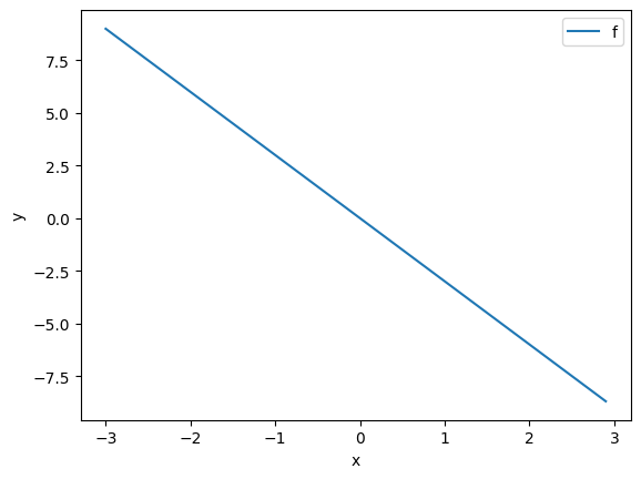
Let us add some noise to the data in order to simulate the real data. Use torch.randn(X.size()) to generate Gaussian noise that is the same size as X and has a standard deviation opf 0.1.
# Add some noise to f(X) and save it in Y

Y = f + 0.1 * torch.randn(X.size())
Plot the Y:
# Plot the data points

plt.plot(X.numpy(), Y.numpy(), 'rx', label = 'Y')

plt.plot(X.numpy(), f.numpy(), label = 'f')
plt.xlabel('x')
plt.ylabel('y')
plt.legend()
plt.show()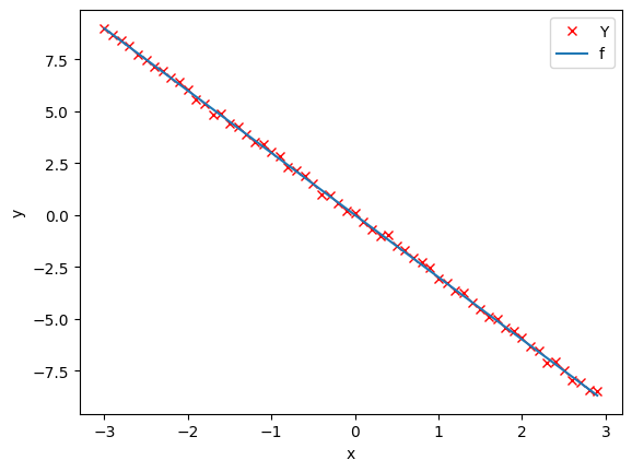
Create the Model and Cost Function (Total Loss)
In this section, let us create the model and the cost function (total loss) we are going to use to train the model and evaluate the result.
First, define the forward function \(y=w*x\). (We will add the bias in the next lab.)
# Create forward function for prediction

def forward(x):
    return w * x
Define the cost or criterion function using MSE (Mean Square Error):
# Create the MSE function for evaluate the result.

def criterion(yhat, y):
    return torch.mean((yhat - y) ** 2)
Define the learning rate lr and an empty list LOSS to record the loss for each iteration:
# Create Learning Rate and an empty list to record the loss for each iteration

lr = 0.1
LOSS = []
Now, we create a model parameter by setting the argument requires_grad to True because the system must learn it.
w = torch.tensor(-10.0, requires_grad = True)Create a plot_diagram object to visualize the data space and the parameter space for each iteration during training:
gradient_plot = plot_diagram(X, Y, w, stop = 5)Train the Model
Let us define a function for training the model. The steps will be described in the comments.
# Define a function for train the model
def train_model(iter):
for epoch in range (iter):
# make the prediction as we learned in the last lab
Yhat = forward(X)
# calculate the iteration
loss = criterion(Yhat,Y)
# plot the diagram for us to have a better idea
# gradient_plot(Yhat, w, loss.item(), epoch)
# store the loss into list
LOSS.append(loss.item())
# backward pass: compute gradient of the loss with respect to all the learnable parameters
loss.backward()
# updata parameters
w.data = w.data - lr * w.grad.data
# zero the gradients before running the backward pass
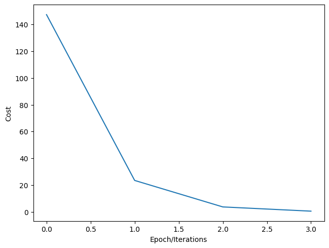
w.grad.data.zero_()Let us try to run 4 iterations of gradient descent:
# Give 4 iterations for training the model here.

train_model(4)
Plot the cost for each iteration:
# Plot the loss for each iteration

plt.plot(LOSS)
plt.tight_layout()
plt.xlabel("Epoch/Iterations")
plt.ylabel("Cost")
Text(38.347222222222214, 0.5, 'Cost')