# Import the libraries we need for this lab

from torch import nn,optim
import torch
import numpy as np
import matplotlib.pyplot as plt

from mpl_toolkits.mplot3d import Axes3D
from torch.utils.data import Dataset, DataLoaderLinear Regression Multiple Outputs
In this lab, you will review how to make a prediction in several different ways by using PyTorch.
Keywords
Training Two Parameter, Mini-Batch Gradient Decent, Training Two Parameter Mini-Batch Gradient Decent

Objective
- How to create a complicated models using pytorch build in functions.
Table of Contents
In this lab, you will create a model the PyTroch way. This will help you more complicated models.
- Make Some Data
- Create the Model and Cost Function the PyTorch way
- Train the Model: Batch Gradient Descent
Estimated Time Needed: 20 min
Preparation
We’ll need the following libraries:
Set the random seed:
# Set the random seed to 1.

torch.manual_seed(1)
<torch._C.Generator at 0x7b084404eeb0>Use this function for plotting:
# The function for plotting 2D

def Plot_2D_Plane(model, dataset, n=0):
    w1 = model.state_dict()['linear.weight'].numpy()[0][0]
    w2 = model.state_dict()['linear.weight'].numpy()[0][1]
    b = model.state_dict()['linear.bias'].numpy()

    # Data
    x1 = data_set.x[:, 0].view(-1, 1).numpy()
    x2 = data_set.x[:, 1].view(-1, 1).numpy()
    y = data_set.y.numpy()

    # Make plane
    X, Y = np.meshgrid(np.arange(x1.min(), x1.max(), 0.05), np.arange(x2.min(), x2.max(), 0.05))
    yhat = w1 * X + w2 * Y + b

    # Plotting
    fig = plt.figure()
    ax = fig.gca(projection='3d')

    ax.plot(x1[:, 0], x2[:, 0], y[:, 0],'ro', label='y') # Scatter plot

    ax.plot_surface(X, Y, yhat) # Plane plot

    ax.set_xlabel('x1 ')
    ax.set_ylabel('x2 ')
    ax.set_zlabel('y')
    plt.title('estimated plane iteration:' + str(n))
    ax.legend()

    plt.show()
Make Some Data
Create a dataset class with two-dimensional features:
# Create a 2D dataset

class Data2D(Dataset):

    # Constructor
    def __init__(self):
        self.x = torch.zeros(20, 2)
        self.x[:, 0] = torch.arange(-1, 1, 0.1)
        self.x[:, 1] = torch.arange(-1, 1, 0.1)
        self.w = torch.tensor([[1.0], [1.0]])
        self.b = 1
        self.f = torch.mm(self.x, self.w) + self.b
        self.y = self.f + 0.1 * torch.randn((self.x.shape[0],1))
        self.len = self.x.shape[0]

    # Getter
    def __getitem__(self, index):
        return self.x[index], self.y[index]

    # Get Length
    def __len__(self):
        return self.len
Create a dataset object:
# Create the dataset object

data_set = Data2D()
Create the Model, Optimizer, and Total Loss Function (Cost)
Create a customized linear regression module:
# Create a customized linear

class LinearRegression(nn.Module):

    # Constructor
    def __init__(self, input_size, output_size):
        super(LinearRegression, self).__init__()
        self.linear = nn.Linear(input_size, output_size)

    # Prediction
    def forward(self, x):
        yhat = self.linear(x)
        return yhat
Create a model. Use two features: make the input size 2 and the output size 1:
# Create the linear regression model and print the parameters

model = LinearRegression(2,1)
print("The parameters: ", list(model.parameters()))
The parameters: [Parameter containing:
tensor([[ 0.6209, -0.1178]], requires_grad=True), Parameter containing:
tensor([0.3026], requires_grad=True)]Create an optimizer object. Set the learning rate to 0.1. Don’t forget to enter the model parameters in the constructor.
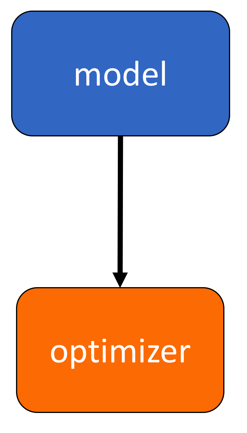
# Create the optimizer

optimizer = optim.SGD(model.parameters(), lr=0.1)
Create the criterion function that calculates the total loss or cost:
# Create the cost function

criterion = nn.MSELoss()
Create a data loader object. Set the batch_size equal to 2:
# Create the data loader

train_loader = DataLoader(dataset=data_set, batch_size=2)
Train the Model via Mini-Batch Gradient Descent
Run 100 epochs of Mini-Batch Gradient Descent and store the total loss or cost for every iteration. Remember that this is an approximation of the true total loss or cost:
# Train the model

LOSS = []
# print("Before Training: ")
# Plot_2D_Plane(model, data_set)
epochs = 100

def train_model(epochs):
    for epoch in range(epochs):
        for x,y in train_loader:
            yhat = model(x)
            loss = criterion(yhat, y)
            LOSS.append(loss.item())
            optimizer.zero_grad()
            loss.backward()
            optimizer.step()
train_model(epochs)
# print("After Training: ")
# Plot_2D_Plane(model, data_set, epochs)
# Plot out the Loss and iteration diagram
plt.plot(LOSS)
plt.xlabel("Iterations ")
plt.ylabel("Cost/total loss ")Text(0, 0.5, 'Cost/total loss ')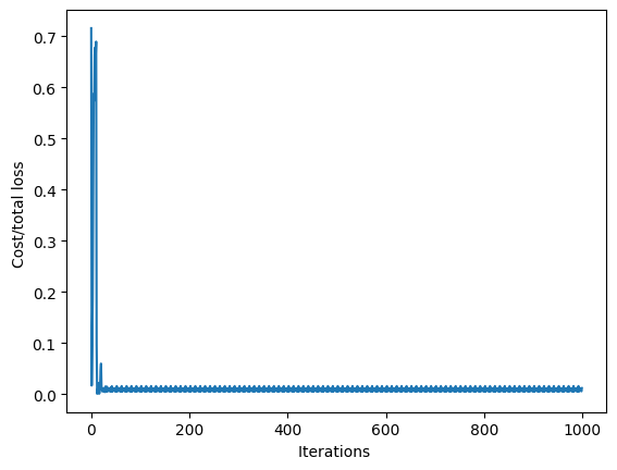
Practice
Create a new model1. Train the model with a batch size 30 and learning rate 0.1, store the loss or total cost in a list LOSS1, and plot the results.
# Practice create model1. Train the model with batch size 30 and learning rate 0.1, store the loss in a list <code>LOSS1</code>. Plot the results.

data_set = Data2D()
Double-click here for the solution.
Use the following validation data to calculate the total loss or cost for both models:
torch.manual_seed(2)

validation_data = Data2D()
Y = validation_data.y
X = validation_data.x