Multiple Channel Convolutional Network

In this lab, you will learn two important components in building a convolutional neural network.

Keywords

Training Two Parameter, Mini-Batch Gradient Decent, Training Two Parameter Mini-Batch Gradient Decent

Photo by DATAIDEA

Objective for this Notebook

1. Learn on Multiple Input and Multiple Output Channels.

Don’t Miss Any Updates!

Before we continue, I have a humble request, to be among the first to hear about future updates of the course materials, simply enter your email below, follow us on (formally Twitter), or subscribe to our YouTube channel.

Import the following libraries:

import torch 
import torch.nn as nn
import matplotlib.pyplot as plt
import numpy as np
from scipy import ndimage, misc

Multiple Output Channels

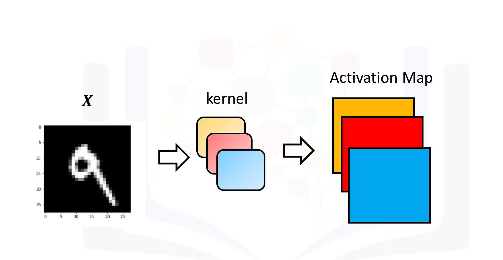
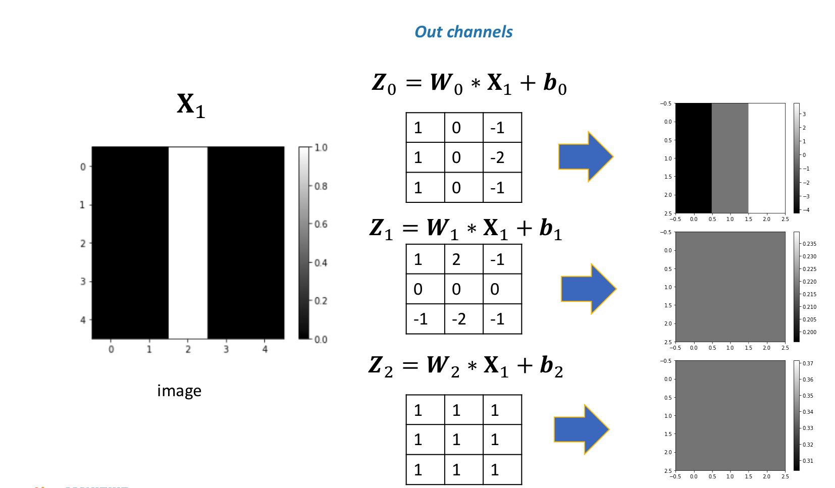
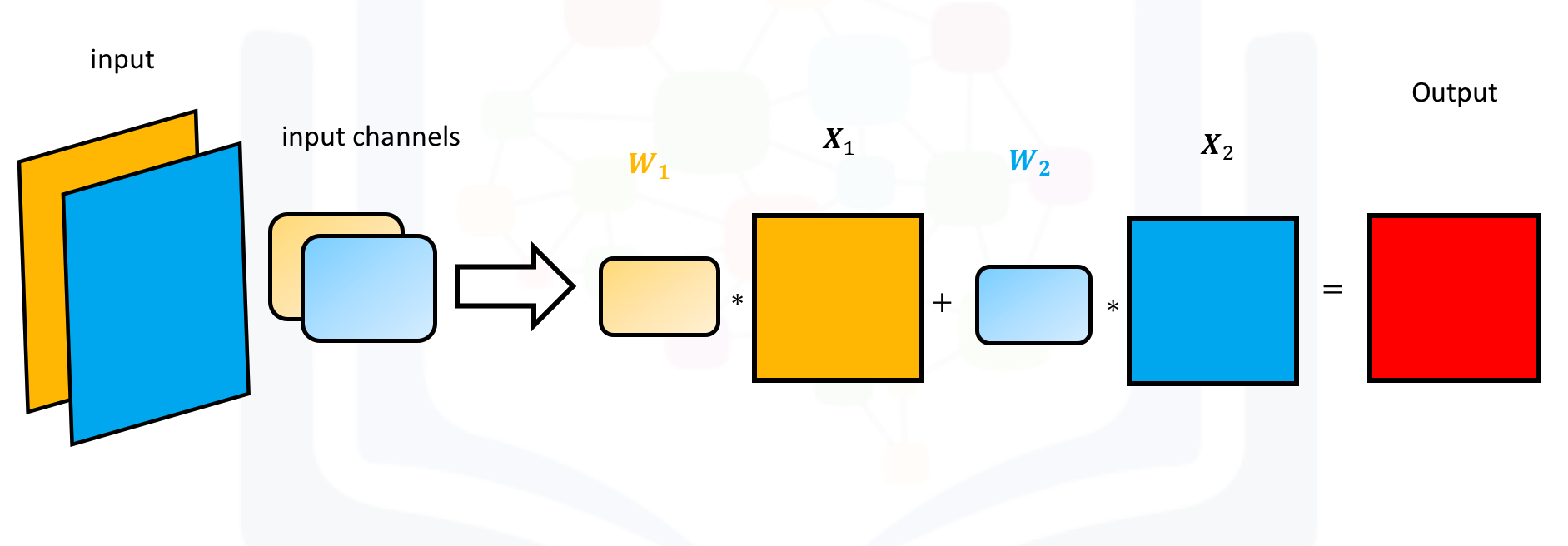
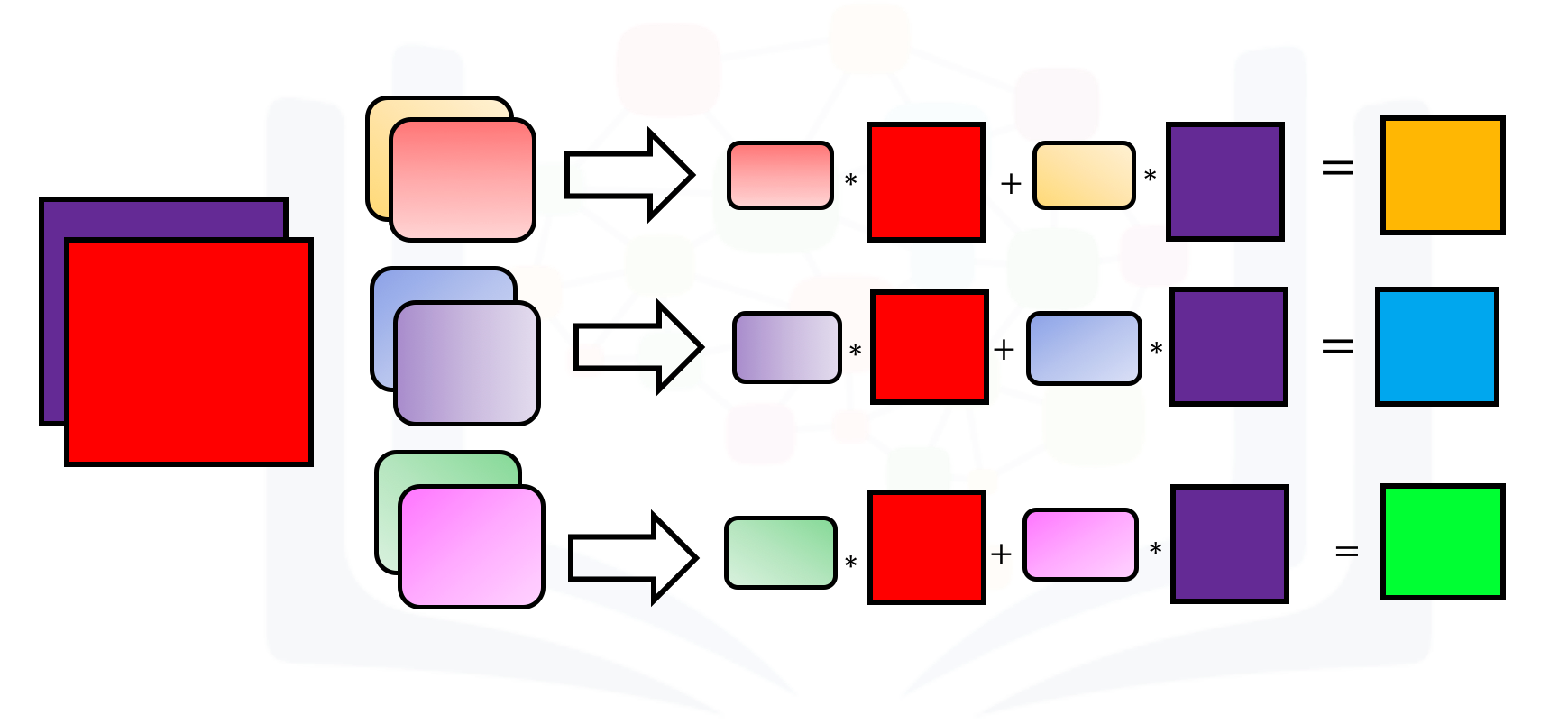
In Pytroch, you can create a Conv2d object with multiple outputs. For each channel, a kernel is created, and each kernel performs a convolution independently. As a result, the number of outputs is equal to the number of channels. This is demonstrated in the following figure. The number 9 is convolved with three kernels: each of a different color. There are three different activation maps represented by the different colors.

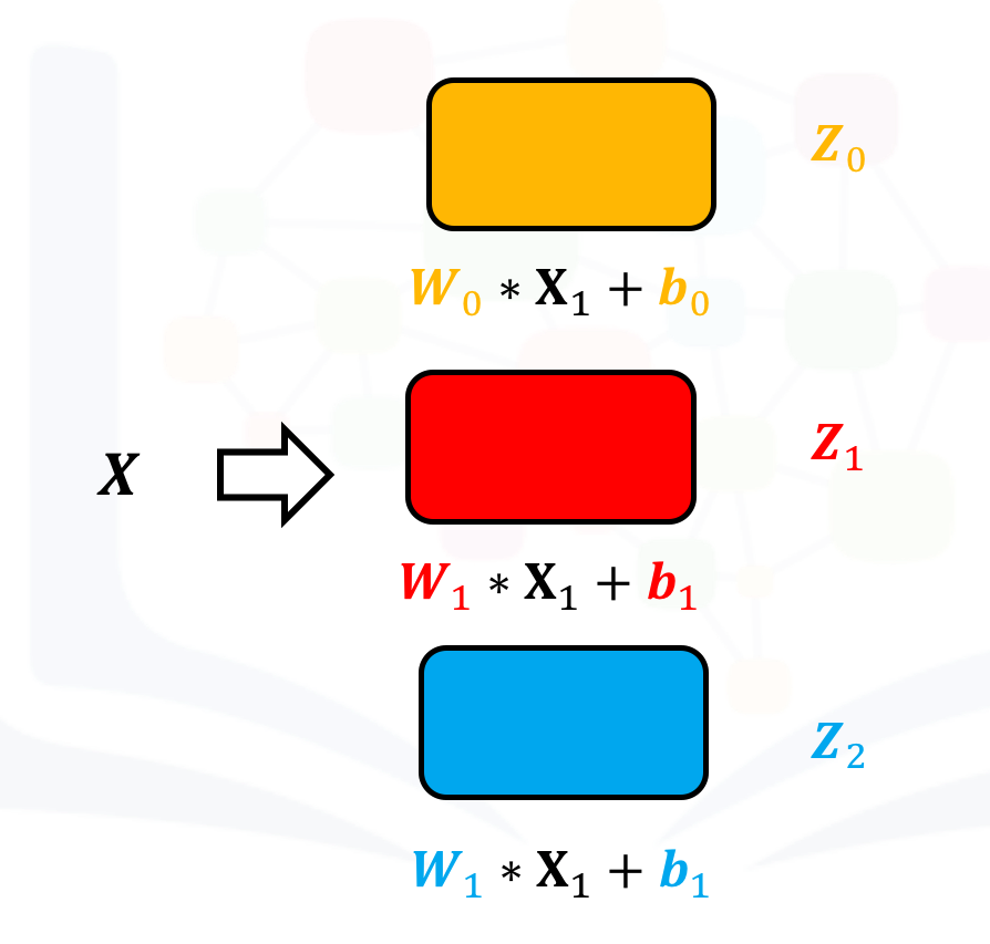
Symbolically, this can be represented as follows:

Create a Conv2d with three channels:

conv1 = nn.Conv2d(in_channels=1, out_channels=3,kernel_size=3)

Pytorch randomly assigns values to each kernel. However, use kernels that have been developed to detect edges:

Gx=torch.tensor([[1.0,0,-1.0],[2.0,0,-2.0],[1.0,0.0,-1.0]])
Gy=torch.tensor([[1.0,2.0,1.0],[0.0,0.0,0.0],[-1.0,-2.0,-1.0]])

conv1.state_dict()['weight'][0][0]=Gx
conv1.state_dict()['weight'][1][0]=Gy
conv1.state_dict()['weight'][2][0]=torch.ones(3,3)

Each kernel has its own bias, so set them all to zero:

conv1.state_dict()['bias'][:]=torch.tensor([0.0,0.0,0.0])
conv1.state_dict()['bias']

tensor([0., 0., 0.])

Print out each kernel:

for x in conv1.state_dict()['weight']:
    print(x)

tensor([[[ 1.,  0., -1.],
         [ 2.,  0., -2.],
         [ 1.,  0., -1.]]])
tensor([[[ 1.,  2.,  1.],
         [ 0.,  0.,  0.],
         [-1., -2., -1.]]])
tensor([[[1., 1., 1.],
         [1., 1., 1.],
         [1., 1., 1.]]])

Create an input image to represent the input X:

image=torch.zeros(1,1,5,5)
image[0,0,:,2]=1
image

tensor([[[[0., 0., 1., 0., 0.],
          [0., 0., 1., 0., 0.],
          [0., 0., 1., 0., 0.],
          [0., 0., 1., 0., 0.],
          [0., 0., 1., 0., 0.]]]])

Plot it as an image:

plt.imshow(image[0,0,:,:].numpy(), interpolation='nearest', cmap=plt.cm.gray)
plt.colorbar()
plt.show()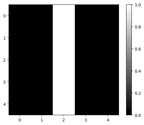

Perform convolution using each channel:

out=conv1(image)

The result is a 1x3x3x3 tensor. This represents one sample with three channels, and each channel contains a 3x3 image. The same rules that govern the shape of each image were discussed in the last section.

out.shape

torch.Size([1, 3, 3, 3])

Print out each channel as a tensor or an image:

for channel,image in enumerate(out[0]):
    plt.imshow(image.detach().numpy(), interpolation='nearest', cmap=plt.cm.gray)
    print(image)
    plt.title("channel {}".format(channel))
    plt.colorbar()
    plt.show()

tensor([[-4.,  0.,  4.],
        [-4.,  0.,  4.],
        [-4.,  0.,  4.]], grad_fn=<UnbindBackward0>)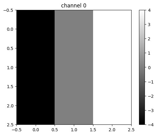

tensor([[0., 0., 0.],
        [0., 0., 0.],
        [0., 0., 0.]], grad_fn=<UnbindBackward0>)

tensor([[3., 3., 3.],
        [3., 3., 3.],
        [3., 3., 3.]], grad_fn=<UnbindBackward0>)

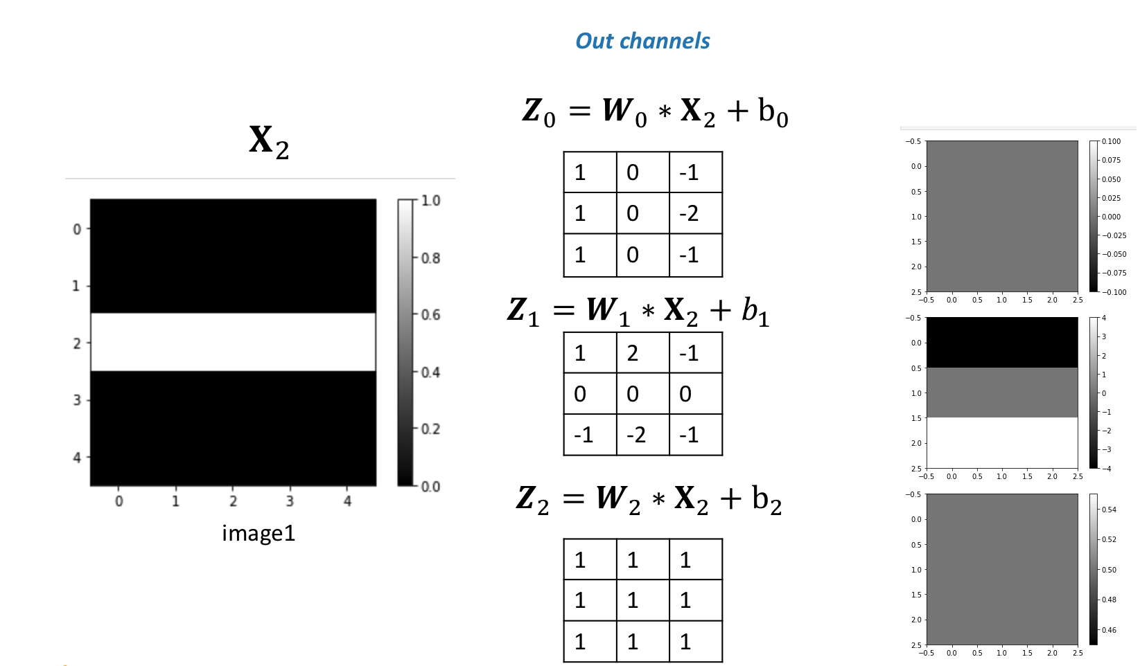
Different kernels can be used to detect various features in an image. You can see that the first channel fluctuates, and the second two channels produce a constant value. The following figure summarizes the process:

If you use a different image, the result will be different:

image1=torch.zeros(1,1,5,5)
image1[0,0,2,:]=1
print(image1)
plt.imshow(image1[0,0,:,:].detach().numpy(), interpolation='nearest', cmap=plt.cm.gray)
plt.show()

tensor([[[[0., 0., 0., 0., 0.],
          [0., 0., 0., 0., 0.],
          [1., 1., 1., 1., 1.],
          [0., 0., 0., 0., 0.],
          [0., 0., 0., 0., 0.]]]])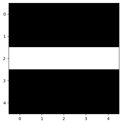

In this case, the second channel fluctuates, and the first and the third channels produce a constant value.

out1=conv1(image1)
for channel,image in enumerate(out1[0]):
    plt.imshow(image.detach().numpy(), interpolation='nearest', cmap=plt.cm.gray)
    print(image)
    plt.title("channel {}".format(channel))
    plt.colorbar()
    plt.show()

tensor([[0., 0., 0.],
        [0., 0., 0.],
        [0., 0., 0.]], grad_fn=<UnbindBackward0>)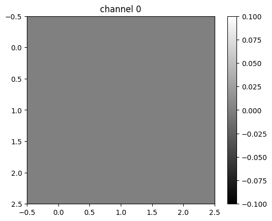

tensor([[-4., -4., -4.],
        [ 0.,  0.,  0.],
        [ 4.,  4.,  4.]], grad_fn=<UnbindBackward0>)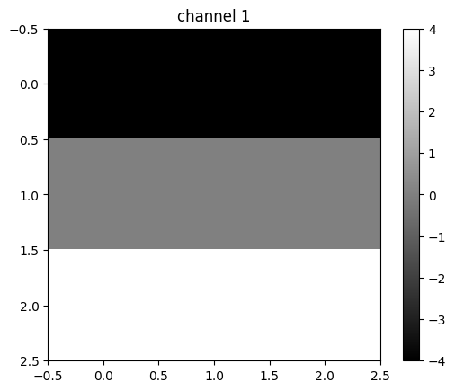

tensor([[3., 3., 3.],
        [3., 3., 3.],
        [3., 3., 3.]], grad_fn=<UnbindBackward0>)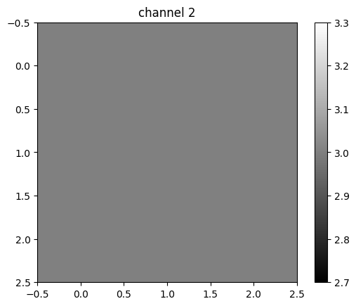

The following figure summarizes the process:

Multiple Input Channels

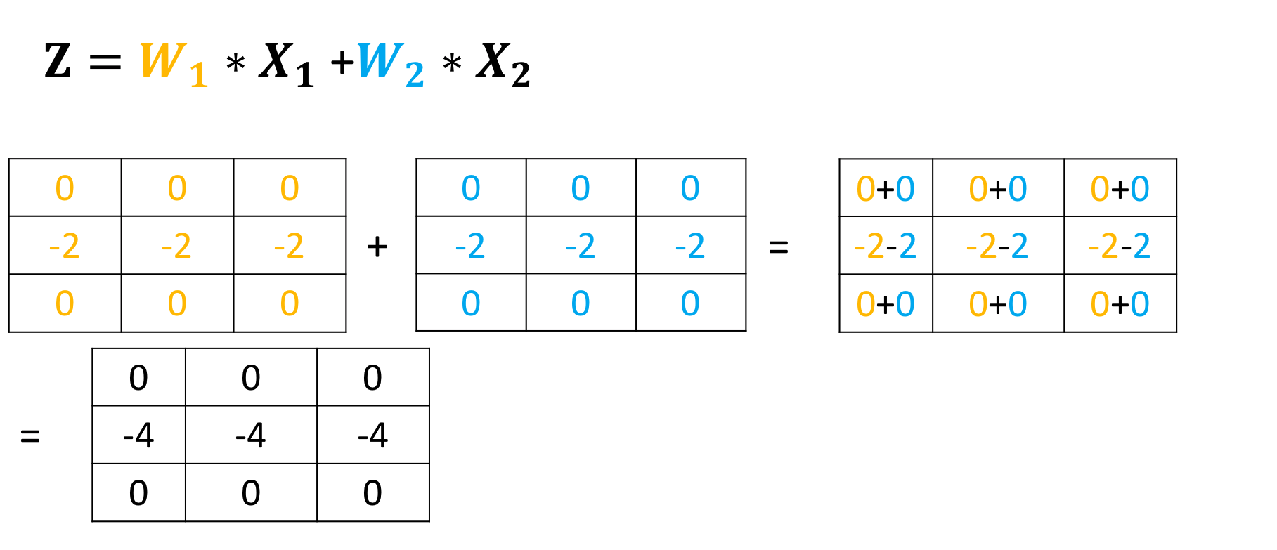
For two inputs, you can create two kernels. Each kernel performs a convolution on its associated input channel. The resulting output is added together as shown:

Create an input with two channels:

image2=torch.zeros(1,2,5,5)
image2[0,0,2,:]=-2
image2[0,1,2,:]=1
image2

tensor([[[[ 0.,  0.,  0.,  0.,  0.],
          [ 0.,  0.,  0.,  0.,  0.],
          [-2., -2., -2., -2., -2.],
          [ 0.,  0.,  0.,  0.,  0.],
          [ 0.,  0.,  0.,  0.,  0.]],

         [[ 0.,  0.,  0.,  0.,  0.],
          [ 0.,  0.,  0.,  0.,  0.],
          [ 1.,  1.,  1.,  1.,  1.],
          [ 0.,  0.,  0.,  0.,  0.],
          [ 0.,  0.,  0.,  0.,  0.]]]])

Plot out each image:

for channel,image in enumerate(image2[0]):
    plt.imshow(image.detach().numpy(), interpolation='nearest', cmap=plt.cm.gray)
    print(image)
    plt.title("channel {}".format(channel))
    plt.colorbar()
    plt.show()

tensor([[ 0.,  0.,  0.,  0.,  0.],
        [ 0.,  0.,  0.,  0.,  0.],
        [-2., -2., -2., -2., -2.],
        [ 0.,  0.,  0.,  0.,  0.],
        [ 0.,  0.,  0.,  0.,  0.]])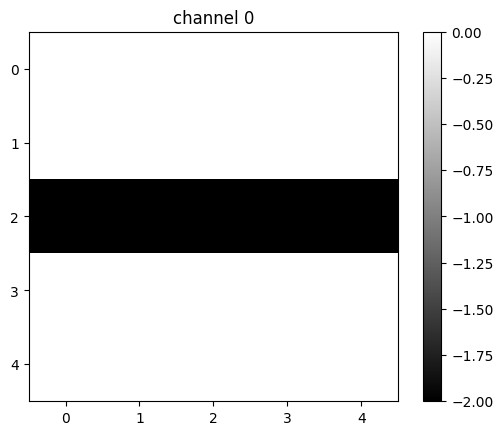

tensor([[0., 0., 0., 0., 0.],
        [0., 0., 0., 0., 0.],
        [1., 1., 1., 1., 1.],
        [0., 0., 0., 0., 0.],
        [0., 0., 0., 0., 0.]])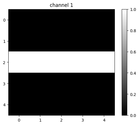

Create a Conv2d object with two inputs:

conv3 = nn.Conv2d(in_channels=2, out_channels=1,kernel_size=3)

Assign kernel values to make the math a little easier:

Gx1=torch.tensor([[0.0,0.0,0.0],[0,1.0,0],[0.0,0.0,0.0]])
conv3.state_dict()['weight'][0][0]=1*Gx1
conv3.state_dict()['weight'][0][1]=-2*Gx1
conv3.state_dict()['bias'][:]=torch.tensor([0.0])

conv3.state_dict()['weight']

tensor([[[[ 0.,  0.,  0.],
          [ 0.,  1.,  0.],
          [ 0.,  0.,  0.]],

         [[-0., -0., -0.],
          [-0., -2., -0.],
          [-0., -0., -0.]]]])

Perform the convolution:

conv3(image2)

tensor([[[[ 0.,  0.,  0.],
          [-4., -4., -4.],
          [ 0.,  0.,  0.]]]], grad_fn=<ConvolutionBackward0>)

The following images summarize the process. The object performs Convolution.

Then, it adds the result:

Multiple Input and Multiple Output Channels

When using multiple inputs and outputs, a kernel is created for each input, and the process is repeated for each output. The process is summarized in the following image.

There are two input channels and 3 output channels. For each channel, the input in red and purple is convolved with an individual kernel that is colored differently. As a result, there are three outputs.

Create an example with two inputs and three outputs and assign the kernel values to make the math a little easier:

conv4 = nn.Conv2d(in_channels=2, out_channels=3,kernel_size=3)
conv4.state_dict()['weight'][0][0]=torch.tensor([[0.0,0.0,0.0],[0,0.5,0],[0.0,0.0,0.0]])
conv4.state_dict()['weight'][0][1]=torch.tensor([[0.0,0.0,0.0],[0,0.5,0],[0.0,0.0,0.0]])


conv4.state_dict()['weight'][1][0]=torch.tensor([[0.0,0.0,0.0],[0,1,0],[0.0,0.0,0.0]])
conv4.state_dict()['weight'][1][1]=torch.tensor([[0.0,0.0,0.0],[0,-1,0],[0.0,0.0,0.0]])

conv4.state_dict()['weight'][2][0]=torch.tensor([[1.0,0,-1.0],[2.0,0,-2.0],[1.0,0.0,-1.0]])
conv4.state_dict()['weight'][2][1]=torch.tensor([[1.0,2.0,1.0],[0.0,0.0,0.0],[-1.0,-2.0,-1.0]])

For each output, there is a bias, so set them all to zero:

conv4.state_dict()['bias'][:]=torch.tensor([0.0,0.0,0.0])

Create a two-channel image and plot the results:

image4=torch.zeros(1,2,5,5)
image4[0][0]=torch.ones(5,5)
image4[0][1][2][2]=1
for channel,image in enumerate(image4[0]):
    plt.imshow(image.detach().numpy(), interpolation='nearest', cmap=plt.cm.gray)
    print(image)
    plt.title("channel {}".format(channel))
    plt.colorbar()
    plt.show()

tensor([[1., 1., 1., 1., 1.],
        [1., 1., 1., 1., 1.],
        [1., 1., 1., 1., 1.],
        [1., 1., 1., 1., 1.],
        [1., 1., 1., 1., 1.]])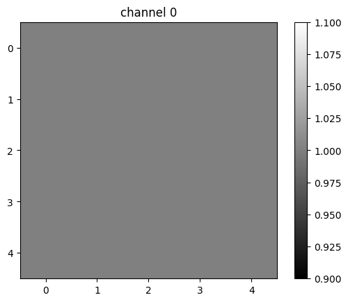

tensor([[0., 0., 0., 0., 0.],
        [0., 0., 0., 0., 0.],
        [0., 0., 1., 0., 0.],
        [0., 0., 0., 0., 0.],
        [0., 0., 0., 0., 0.]])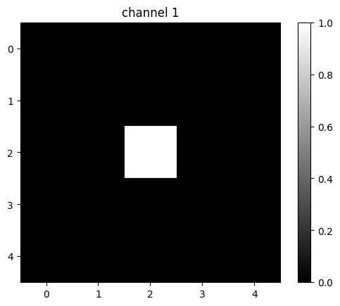

Perform the convolution:

z=conv4(image4)
z

tensor([[[[ 0.5000,  0.5000,  0.5000],
          [ 0.5000,  1.0000,  0.5000],
          [ 0.5000,  0.5000,  0.5000]],

         [[ 1.0000,  1.0000,  1.0000],
          [ 1.0000,  0.0000,  1.0000],
          [ 1.0000,  1.0000,  1.0000]],

         [[-1.0000, -2.0000, -1.0000],
          [ 0.0000,  0.0000,  0.0000],
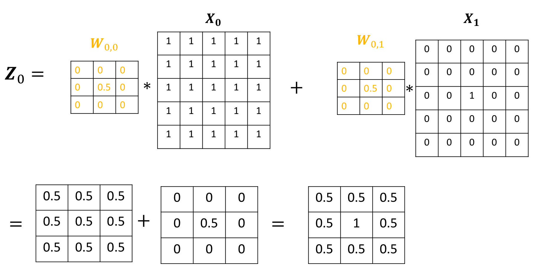
          [ 1.0000,  2.0000,  1.0000]]]], grad_fn=<ConvolutionBackward0>)

The output of the first channel is given by:

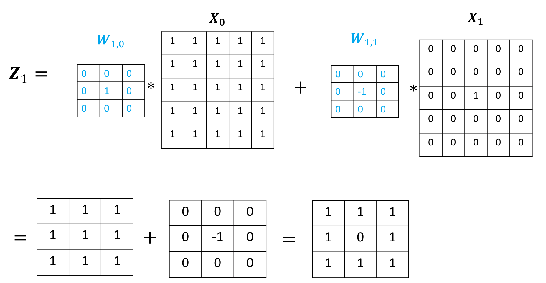
The output of the second channel is given by:

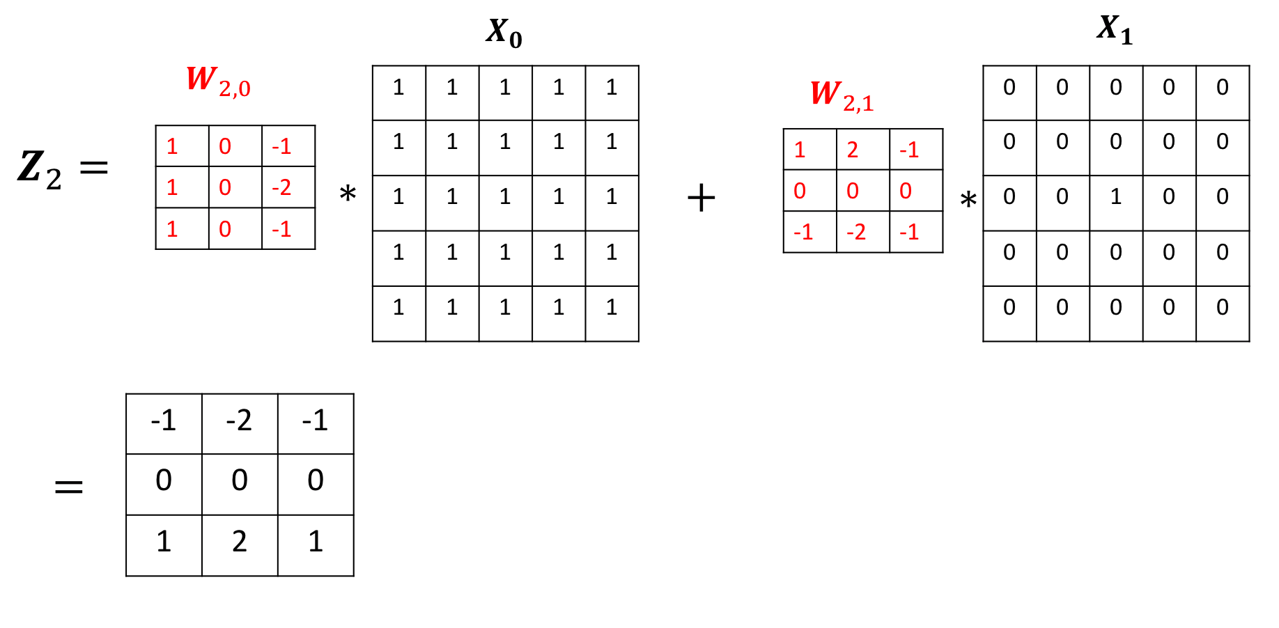
The output of the third channel is given by:

Practice Questions

Use the following two convolution objects to produce the same result as two input channel convolution on imageA and imageB as shown in the following image:

imageA=torch.zeros(1,1,5,5)
imageB=torch.zeros(1,1,5,5)
imageA[0,0,2,:]=-2
imageB[0,0,2,:]=1


conv5 = nn.Conv2d(in_channels=1, out_channels=1,kernel_size=3)
conv6 = nn.Conv2d(in_channels=1, out_channels=1,kernel_size=3)


Gx1=torch.tensor([[0.0,0.0,0.0],[0,1.0,0],[0.0,0.0,0.0]])
conv5.state_dict()['weight'][0][0]=1*Gx1
conv6.state_dict()['weight'][0][0]=-2*Gx1
conv5.state_dict()['bias'][:]=torch.tensor([0.0])
conv6.state_dict()['bias'][:]=torch.tensor([0.0])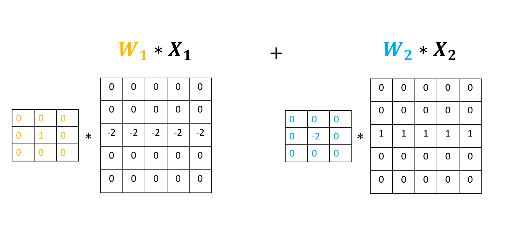

Double-click here for the solution.

What’s on your mind? Put it in the comments!