Logistic Regression

In this lab, we will cover logistic regression using PyTorch.

Author

Juma Shafara

Published

August 8, 2024

Keywords

Training Two Parameter, Mini-Batch Gradient Decent, Training Two Parameter Mini-Batch Gradient Decent

Objective

How to create a logistic regression object with the nn.Sequential model.

In this lab, we will cover logistic regression using PyTorch.

Logistic Function
Build a Logistic Regression Using nn.Sequential
Build Custom Modules

Estimated Time Needed: 15 min

Preparation

We’ll need the following libraries:

# Import the libraries we need for this lab

import torch.nn as nn
import torch
import matplotlib.pyplot as plt

Set the random seed:

# Set the random seed

torch.manual_seed(2)

<torch._C.Generator at 0x714cbc14af50>

Logistic Function

Create a tensor ranging from -100 to 100:

z = torch.arange(-100, 100, 0.1).view(-1, 1)
print("The tensor: ", z)

The tensor:  tensor([[-100.0000],
        [ -99.9000],
        [ -99.8000],
        ...,
        [  99.7000],
        [  99.8000],
        [  99.9000]])

Create a sigmoid object:

# Create sigmoid object

sig = nn.Sigmoid()

Apply the element-wise function Sigmoid with the object:

# Use sigmoid object to calculate the 

yhat = sig(z)

Plot the results:

plt.plot(z.numpy(), yhat.numpy())
plt.xlabel('z')
plt.ylabel('yhat')

Text(0, 0.5, 'yhat')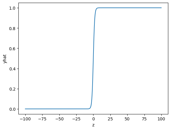

Apply the element-wise Sigmoid from the function module and plot the results:

yhat = torch.sigmoid(z)
plt.plot(z.numpy(), yhat.numpy())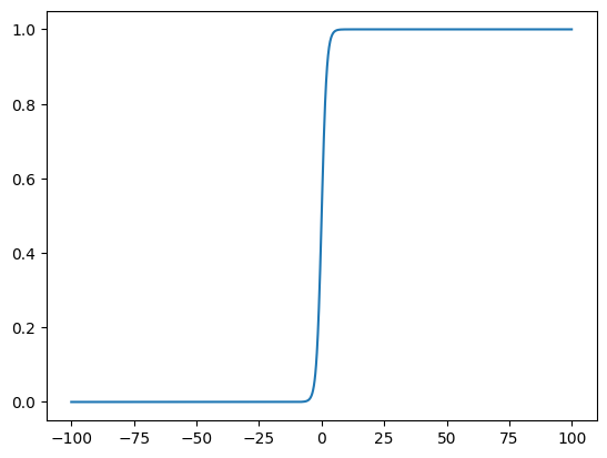

Build a Logistic Regression with `nn.Sequential`

Create a 1x1 tensor where x represents one data sample with one dimension, and 2x1 tensor X represents two data samples of one dimension:

# Create x and X tensor

x = torch.tensor([[1.0]])
X = torch.tensor([[1.0], [100]])
print('x = ', x)
print('X = ', X)

x =  tensor([[1.]])
X =  tensor([[  1.],
        [100.]])

Create a logistic regression object with the nn.Sequential model with a one-dimensional input:

# Use sequential function to create model

model = nn.Sequential(nn.Linear(1, 1), nn.Sigmoid())

The object is represented in the following diagram:

In this case, the parameters are randomly initialized. You can view them the following ways:

# Print the parameters

print("list(model.parameters()):\n ", list(model.parameters()))
print("\nmodel.state_dict():\n ", model.state_dict())

list(model.parameters()):
  [Parameter containing:
tensor([[-0.5717,  0.1614]], requires_grad=True), Parameter containing:
tensor([-0.6260], requires_grad=True)]

model.state_dict():
  OrderedDict({'linear.weight': tensor([[-0.5717,  0.1614]]), 'linear.bias': tensor([-0.6260])})

Make a prediction with one sample:

# The prediction for x

yhat = model(x)
print("The prediction: ", yhat)

The prediction:  tensor([[0.2943]], grad_fn=<SigmoidBackward0>)

Calling the object with tensor X performed the following operation (code values may not be the same as the diagrams value depending on the version of PyTorch) :

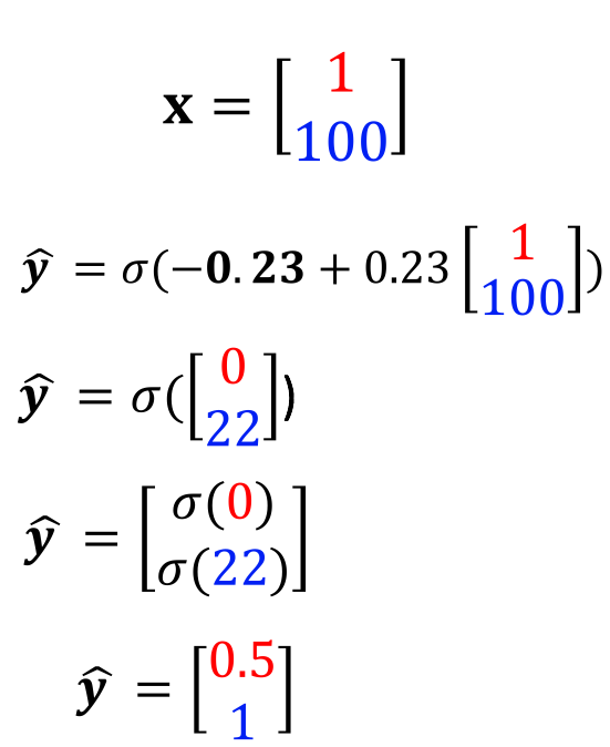
Make a prediction with multiple samples:

# The prediction for X

yhat = model(X)
yhat

tensor([[0.4979],
        [1.0000]], grad_fn=<SigmoidBackward0>)

Calling the object performed the following operation:

Create a 1x2 tensor where x represents one data sample with one dimension, and 2x3 tensor X represents one data sample of two dimensions:

# Create and print samples

x = torch.tensor([[1.0, 1.0]])
X = torch.tensor([[1.0, 1.0], [1.0, 2.0], [1.0, 3.0]])
print('x = ', x)
print('X = ', X)

x =  tensor([[1., 1.]])
X =  tensor([[1., 1.],
        [1., 2.],
        [1., 3.]])

Create a logistic regression object with the nn.Sequential model with a two-dimensional input:

# Create new model using nn.sequential()

model = nn.Sequential(nn.Linear(2, 1), nn.Sigmoid())

The object will apply the Sigmoid function to the output of the linear function as shown in the following diagram:

In this case, the parameters are randomly initialized. You can view them the following ways:

# Print the parameters

print("list(model.parameters()):\n ", list(model.parameters()))
print("\nmodel.state_dict():\n ", model.state_dict())

list(model.parameters()):
  [Parameter containing:
tensor([[ 0.1939, -0.0361]], requires_grad=True), Parameter containing:
tensor([0.3021], requires_grad=True)]

model.state_dict():
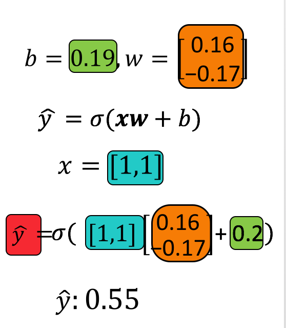
  OrderedDict({'0.weight': tensor([[ 0.1939, -0.0361]]), '0.bias': tensor([0.3021])})

Make a prediction with one sample:

# Make the prediction of x

yhat = model(x)
print("The prediction: ", yhat)

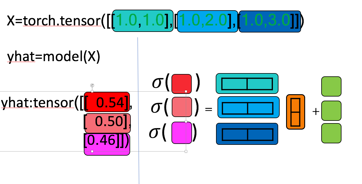
The prediction:  tensor([[0.6130]], grad_fn=<SigmoidBackward0>)

The operation is represented in the following diagram:

Make a prediction with multiple samples:

# The prediction of X

yhat = model(X)
print("The prediction: ", yhat)

The prediction:  tensor([[0.6130],
        [0.6044],
        [0.5957]], grad_fn=<SigmoidBackward0>)

The operation is represented in the following diagram:

Build Custom Modules

In this section, you will build a custom Module or class. The model or object function is identical to using nn.Sequential.

Create a logistic regression custom module:

# Create logistic_regression custom class

class logistic_regression(nn.Module):
    
    # Constructor
    def __init__(self, n_inputs):
        super(logistic_regression, self).__init__()
        self.linear = nn.Linear(n_inputs, 1)
    
    # Prediction
    def forward(self, x):
        yhat = torch.sigmoid(self.linear(x))
        return yhat

Create a 1x1 tensor where x represents one data sample with one dimension, and 3x1 tensor where \(X\) represents one data sample of one dimension:

# Create x and X tensor

x = torch.tensor([[1.0]])
X = torch.tensor([[-100], [0], [100.0]])
print('x = ', x)
print('X = ', X)

x =  tensor([[1.]])
X =  tensor([[-100.],
        [   0.],
        [ 100.]])

Create a model to predict one dimension:

# Create logistic regression model

model = logistic_regression(1)

In this case, the parameters are randomly initialized. You can view them the following ways:

# Print parameters 

print("list(model.parameters()):\n ", list(model.parameters()))
print("\nmodel.state_dict():\n ", model.state_dict())

list(model.parameters()):
  [Parameter containing:
tensor([[0.2381]], requires_grad=True), Parameter containing:
tensor([-0.1149], requires_grad=True)]

model.state_dict():
  OrderedDict({'linear.weight': tensor([[0.2381]]), 'linear.bias': tensor([-0.1149])})

Make a prediction with one sample:

# Make the prediction of x

yhat = model(x)
print("The prediction result: \n", yhat)

The prediction result: 
 tensor([[0.5307]], grad_fn=<SigmoidBackward0>)

Make a prediction with multiple samples:

# Make the prediction of X

yhat = model(X)
print("The prediction result: \n", yhat)

The prediction result: 
 tensor([[4.0805e-11],
        [4.7130e-01],
        [1.0000e+00]], grad_fn=<SigmoidBackward0>)

Create a logistic regression object with a function with two inputs:

# Create logistic regression model

model = logistic_regression(2)

Create a 1x2 tensor where x represents one data sample with one dimension, and 3x2 tensor X represents one data sample of one dimension:

# Create x and X tensor

x = torch.tensor([[1.0, 2.0]])
X = torch.tensor([[100, -100], [0.0, 0.0], [-100, 100]])
print('x = ', x)
print('X = ', X)

x =  tensor([[1., 2.]])
X =  tensor([[ 100., -100.],
        [   0.,    0.],
        [-100.,  100.]])

Make a prediction with one sample:

# Make the prediction of x

yhat = model(x)
print("The prediction result: \n", yhat)

The prediction result: 
 tensor([[0.2943]], grad_fn=<SigmoidBackward0>)

Make a prediction with multiple samples:

# Make the prediction of X

yhat = model(X)
print("The prediction result: \n", yhat)

The prediction result: 
 tensor([[7.7529e-33],
        [3.4841e-01],
        [1.0000e+00]], grad_fn=<SigmoidBackward0>)

Practice

Make your own model my_model as applying linear regression first and then logistic regression using nn.Sequential(). Print out your prediction.

# Practice: Make your model and make the prediction

X = torch.tensor([-10.0])

my_model = nn.Sequential(nn.Linear(1, 1), nn.Sigmoid())

my_model(X)

tensor([0.2231], grad_fn=<SigmoidBackward0>)

Double-click here for the solution.

About the Author:

Hi, My name is Juma Shafara. Am a Data Scientist and Instructor at DATAIDEA. I have taught hundreds of peope Programming, Data Analysis and Machine Learning.

I also enjoy developing innovative algorithms and models that can drive insights and value.

I regularly share some content that I find useful throughout my learning/teaching journey to simplify concepts in Machine Learning, Mathematics, Programming, and related topics on my website jumashafara.dataidea.org.

Besides these technical stuff, I enjoy watching soccer, movies and reading mystery books.

Logistic Regression

Objective

Table of Contents

Preparation

Logistic Function

Build a Logistic Regression with `nn.Sequential`

Build Custom Modules

Practice

About the Author:

What’s on your mind? Put it in the comments!

Objective

Table of Contents

Preparation

Logistic Function

Build a Logistic Regression with nn.Sequential

Build Custom Modules

Practice

About the Author:

What’s on your mind? Put it in the comments!

Build a Logistic Regression with `nn.Sequential`