Simple Convolutional Neural Network

In this lab, we will use a Convolutional Neral Networks to classify horizontal an vertical Lines

Keywords

Training Two Parameter, Mini-Batch Gradient Decent, Training Two Parameter Mini-Batch Gradient Decent

Photo by DATAIDEA

Objective for this Notebook

1. Learn Convolutional Neral Network

2. Define Softmax , Criterion function, Optimizer and Train the Model

Don’t Miss Any Updates!

Before we continue, I have a humble request, to be among the first to hear about future updates of the course materials, simply enter your email below, follow us on (formally Twitter), or subscribe to our YouTube channel.

Helper functions

import torch 
import torch.nn as nn
import torchvision.transforms as transforms
import torchvision.datasets as dsets
import matplotlib.pylab as plt
import numpy as np
import pandas as pd

torch.manual_seed(4)

<torch._C.Generator at 0x70243022eeb0>

function to plot out the parameters of the Convolutional layers

def plot_channels(W):
    #number of output channels 
    n_out=W.shape[0]
    #number of input channels 
    n_in=W.shape[1]
    w_min=W.min().item()
    w_max=W.max().item()
    fig, axes = plt.subplots(n_out,n_in)
    fig.subplots_adjust(hspace = 0.1)
    out_index=0
    in_index=0
    #plot outputs as rows inputs as columns 
    for ax in axes.flat:
    
        if in_index>n_in-1:
            out_index=out_index+1
            in_index=0
              
        ax.imshow(W[out_index,in_index,:,:], vmin=w_min, vmax=w_max, cmap='seismic')
        ax.set_yticklabels([])
        ax.set_xticklabels([])
        in_index=in_index+1

    plt.show()

show_data: plot out data sample

def show_data(dataset,sample):

    plt.imshow(dataset.x[sample,0,:,:].numpy(),cmap='gray')
    plt.title('y='+str(dataset.y[sample].item()))
    plt.show()

create some toy data

from torch.utils.data import Dataset, DataLoader
class Data(Dataset):
    def __init__(self,N_images=100,offset=0,p=0.9, train=False):
        """
        p:portability that pixel is wight  
        N_images:number of images 
        offset:set a random vertical and horizontal offset images by a sample should be less than 3 
        """
        if train==True:
            np.random.seed(1)  
        
        #make images multiple of 3 
        N_images=2*(N_images//2)
        images=np.zeros((N_images,1,11,11))
        start1=3
        start2=1
        self.y=torch.zeros(N_images).type(torch.long)

        for n in range(N_images):
            if offset>0:
        
                low=int(np.random.randint(low=start1, high=start1+offset, size=1))
                high=int(np.random.randint(low=start2, high=start2+offset, size=1))
            else:
                low=4
                high=1
        
            if n<=N_images//2:
                self.y[n]=0
                images[n,0,high:high+9,low:low+3]= np.random.binomial(1, p, (9,3))
            elif  n>N_images//2:
                self.y[n]=1
                images[n,0,low:low+3,high:high+9] = np.random.binomial(1, p, (3,9))
           
        
        
        self.x=torch.from_numpy(images).type(torch.FloatTensor)
        self.len=self.x.shape[0]
        del(images)
        np.random.seed(0)
    def __getitem__(self,index):      
        return self.x[index],self.y[index]
    def __len__(self):
        return self.len

plot_activation: plot out the activations of the Convolutional layers

def plot_activations(A,number_rows= 1,name=""):
    A=A[0,:,:,:].detach().numpy()
    n_activations=A.shape[0]
    
    
    print(n_activations)
    A_min=A.min().item()
    A_max=A.max().item()

    if n_activations==1:

        # Plot the image.
        plt.imshow(A[0,:], vmin=A_min, vmax=A_max, cmap='seismic')

    else:
        fig, axes = plt.subplots(number_rows, n_activations//number_rows)
        fig.subplots_adjust(hspace = 0.4)
        for i,ax in enumerate(axes.flat):
            if i< n_activations:
                # Set the label for the sub-plot.
                ax.set_xlabel( "activation:{0}".format(i+1))

                # Plot the image.
                ax.imshow(A[i,:], vmin=A_min, vmax=A_max, cmap='seismic')
                ax.set_xticks([])
                ax.set_yticks([])
    plt.show()

Utility function for computing output of convolutions takes a tuple of (h,w) and returns a tuple of (h,w)

def conv_output_shape(h_w, kernel_size=1, stride=1, pad=0, dilation=1):
    #by Duane Nielsen
    from math import floor
    if type(kernel_size) is not tuple:
        kernel_size = (kernel_size, kernel_size)
    h = floor( ((h_w[0] + (2 * pad) - ( dilation * (kernel_size[0] - 1) ) - 1 )/ stride) + 1)
    w = floor( ((h_w[1] + (2 * pad) - ( dilation * (kernel_size[1] - 1) ) - 1 )/ stride) + 1)
    return h, w

Prepare Data

Load the training dataset with 10000 samples

N_images=10000
train_dataset=Data(N_images=N_images)

Load the testing dataset

validation_dataset=Data(N_images=1000,train=False)
validation_dataset

<__main__.Data at 0x7023c545ee10>

we can see the data type is long

Data Visualization

Each element in the rectangular tensor corresponds to a number representing a pixel intensity as demonstrated by the following image.

We can print out the third label

show_data(train_dataset,0)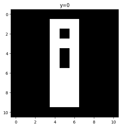

show_data(train_dataset,N_images//2+2)

we can plot the 3rd sample

### Build a Convolutional Neral Network Class

The input image is 11 x11, the following will change the size of the activations:

convolutional layer

max pooling layer

convolutional layer

max pooling layer

with the following parameters kernel_size, stride and pad. We use the following lines of code to change the image before we get tot he fully connected layer

out=conv_output_shape((11,11), kernel_size=2, stride=1, pad=0, dilation=1)
print(out)
out1=conv_output_shape(out, kernel_size=2, stride=1, pad=0, dilation=1)
print(out1)
out2=conv_output_shape(out1, kernel_size=2, stride=1, pad=0, dilation=1)
print(out2)

out3=conv_output_shape(out2, kernel_size=2, stride=1, pad=0, dilation=1)
print(out3)

(10, 10)
(9, 9)
(8, 8)
(7, 7)

Build a Convolutional Network class with two Convolutional layers and one fully connected layer. Pre-determine the size of the final output matrix. The parameters in the constructor are the number of output channels for the first and second layer.

class CNN(nn.Module):
    def __init__(self,out_1=2,out_2=1):
        
        super(CNN,self).__init__()
        #first Convolutional layers 
        self.cnn1=nn.Conv2d(in_channels=1,out_channels=out_1,kernel_size=2,padding=0)
        self.maxpool1=nn.MaxPool2d(kernel_size=2 ,stride=1)

        #second Convolutional layers
        self.cnn2=nn.Conv2d(in_channels=out_1,out_channels=out_2,kernel_size=2,stride=1,padding=0)
        self.maxpool2=nn.MaxPool2d(kernel_size=2 ,stride=1)
        #max pooling 

        #fully connected layer 
        self.fc1=nn.Linear(out_2*7*7,2)
        
    def forward(self,x):
        #first Convolutional layers
        x=self.cnn1(x)
        #activation function 
        x=torch.relu(x)
        #max pooling 
        x=self.maxpool1(x)
        #first Convolutional layers
        x=self.cnn2(x)
        #activation function
        x=torch.relu(x)
        #max pooling
        x=self.maxpool2(x)
        #flatten output 
        x=x.view(x.size(0),-1)
        #fully connected layer
        x=self.fc1(x)
        return x
    
    def activations(self,x):
        #outputs activation this is not necessary just for fun 
        z1=self.cnn1(x)
        a1=torch.relu(z1)
        out=self.maxpool1(a1)
        
        z2=self.cnn2(out)
        a2=torch.relu(z2)
        out=self.maxpool2(a2)
        out=out.view(out.size(0),-1)
        return z1,a1,z2,a2,out

Define the Convolutional Neral Network Classifier , Criterion function, Optimizer and Train the Model

There are 2 output channels for the first layer, and 1 outputs channel for the second layer

model=CNN(2,1)

we can see the model parameters with the object

model

CNN(
  (cnn1): Conv2d(1, 2, kernel_size=(2, 2), stride=(1, 1))
  (maxpool1): MaxPool2d(kernel_size=2, stride=1, padding=0, dilation=1, ceil_mode=False)
  (cnn2): Conv2d(2, 1, kernel_size=(2, 2), stride=(1, 1))
  (maxpool2): MaxPool2d(kernel_size=2, stride=1, padding=0, dilation=1, ceil_mode=False)
  (fc1): Linear(in_features=49, out_features=2, bias=True)
)

Plot the model parameters for the kernels before training the kernels. The kernels are initialized randomly.

plot_channels(model.state_dict()['cnn1.weight'])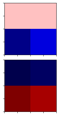

Loss function

plot_channels(model.state_dict()['cnn2.weight'])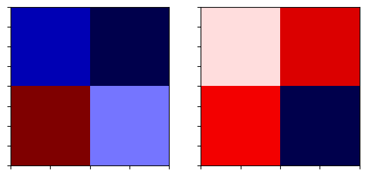

Define the loss function

criterion=nn.CrossEntropyLoss()

optimizer class

learning_rate=0.001

optimizer = torch.optim.Adam(model.parameters(), lr=learning_rate)

Define the optimizer class

train_loader=torch.utils.data.DataLoader(dataset=train_dataset,batch_size=10)
validation_loader=torch.utils.data.DataLoader(dataset=validation_dataset,batch_size=20)

Train the model and determine validation accuracy technically test accuracy (This may take a long time)

n_epochs=10
cost_list=[]
accuracy_list=[]
N_test=len(validation_dataset)
cost=0
#n_epochs
for epoch in range(n_epochs):
    cost=0    
    for x, y in train_loader:
      

        #clear gradient 
        optimizer.zero_grad()
        #make a prediction 
        z=model(x)
        # calculate loss 
        loss=criterion(z,y)
        # calculate gradients of parameters 
        loss.backward()
        # update parameters 
        optimizer.step()
        cost+=loss.item()
    cost_list.append(cost)
        
        
    correct=0
    #perform a prediction on the validation  data  
    for x_test, y_test in validation_loader:

        z=model(x_test)
        _,yhat=torch.max(z.data,1)

        correct+=(yhat==y_test).sum().item()
        

    accuracy=correct/N_test

    accuracy_list.append(accuracy)

Analyse Results

Plot the loss and accuracy on the validation data:

fig, ax1 = plt.subplots()
color = 'tab:red'
ax1.plot(cost_list,color=color)
ax1.set_xlabel('epoch',color=color)
ax1.set_ylabel('total loss',color=color)
ax1.tick_params(axis='y', color=color)
    
ax2 = ax1.twinx()  
color = 'tab:blue'
ax2.set_ylabel('accuracy', color=color)  
ax2.plot( accuracy_list, color=color)
ax2.tick_params(axis='y', labelcolor=color)
fig.tight_layout()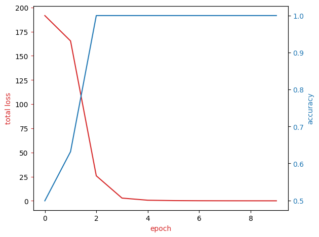

View the results of the parameters for the Convolutional layers

model.state_dict()['cnn1.weight']

tensor([[[[ 0.3507,  0.4734],
          [-0.1160, -0.1536]]],


        [[[-0.4187, -0.2707],
          [ 0.9412,  0.8749]]]])

plot_channels(model.state_dict()['cnn1.weight'])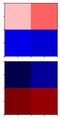

model.state_dict()['cnn1.weight']

tensor([[[[ 0.3507,  0.4734],
          [-0.1160, -0.1536]]],


        [[[-0.4187, -0.2707],
          [ 0.9412,  0.8749]]]])

plot_channels(model.state_dict()['cnn2.weight'])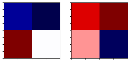

Consider the following sample

show_data(train_dataset,N_images//2+2)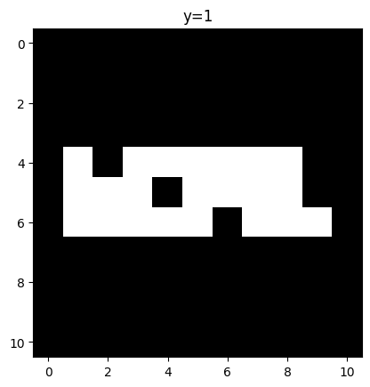

Determine the activations

out=model.activations(train_dataset[N_images//2+2][0].view(1,1,11,11))
out=model.activations(train_dataset[0][0].view(1,1,11,11))

Plot them out

plot_activations(out[0],number_rows=1,name=" feature map")
plt.show()

2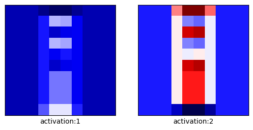

plot_activations(out[2],number_rows=1,name="2nd feature map")
plt.show()

1

plot_activations(out[3],number_rows=1,name="first feature map")
plt.show()

1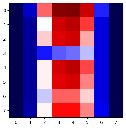

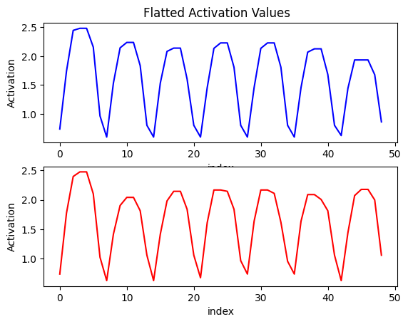
we save the output of the activation after flattening

out1=out[4][0].detach().numpy()

we can do the same for a sample where y=0

out0=model.activations(train_dataset[100][0].view(1,1,11,11))[4][0].detach().numpy()
out0

array([0.7374982 , 1.7757462 , 2.398145  , 2.4768693 , 2.4768693 ,
       2.1022153 , 1.0242625 , 0.6254372 , 1.4152323 , 1.9039373 ,
       2.0423164 , 2.0423164 , 1.8148925 , 1.0581893 , 0.6254372 ,
       1.4152323 , 1.9821635 , 2.1456885 , 2.1456885 , 1.8400384 ,
       1.0581893 , 0.67411214, 1.6115171 , 2.1684833 , 2.1684833 ,
       2.1456885 , 1.8400384 , 0.96484905, 0.7374982 , 1.6366628 ,
       2.1684833 , 2.1684833 , 2.1105773 , 1.618608  , 0.95454437,
       0.7374982 , 1.6366628 , 2.0902567 , 2.0902567 , 2.0072055 ,
       1.8148925 , 1.0581893 , 0.6254372 , 1.4422549 , 2.0730698 ,
       2.178489  , 2.178489  , 1.99857   , 1.0581893 ], dtype=float32)

plt.subplot(2, 1, 1)
plt.plot( out1, 'b')
plt.title('Flatted Activation Values  ')
plt.ylabel('Activation')
plt.xlabel('index')
plt.subplot(2, 1, 2)
plt.plot(out0, 'r')
plt.xlabel('index')
plt.ylabel('Activation')

Text(0, 0.5, 'Activation')

What’s on your mind? Put it in the comments!